Final Project: Design of an Electric Vehicle

• ELECTRIC VEHICLE:

• AIM:

The main of the project is to create a MATLAB model of electric car which uses a battery and a DC motor.

• OBJECTIVE:

INTRODUCTION:

Electric vehicles are becoming increasingly important as not only do they reduce noise and pollution, but also they can be used to reduce the dependence of transport on oil – providing that the power is generated from fuels other than oil. Electric vehicles can also be used to reduce carbon emissions. Production of zero release of carbon dioxide requires that the energy for electric vehicles is produced from non-fossil-fuel sources such as nuclear and alternative energy.

The worst scenario is that we have only 40 years supply of oil left at current usage rates.In practice, of course, increasing scarcity will result in huge price rises and eventually the use of oil and other fossil fuels will not be economically viable, hence oil will be conserved as usage will decrease. Oil can also be produced from other fossil fuels such as coal. Traditionally oil produced in this way was considered to be around 10% more expensive, but with current oil prices production from coal is starting to become economic. Coal is more abundant than oil and there is in excess of 100 years of coal left, though it is still a finite resource.

Increasing worries about global warming continue. Global warming is blamed on the release of carbon dioxide when fossil fuels are burnt and it is believed to give rise to a myriad of problems including climate change and rising sea levels which could destroy many of the world’s coastal cities.

Electric trains are well developed and are widely used whereas road transport has only just reached the point where vehicle manufacturers are starting to produce electric cars in quantity. Whereas small electric vehicles used in niche markets, such as electric bicycles, invalid carriages and golf buggies, are widely used, electric road vehicles are not. Electric road vehicles have not enjoyed the enormous success of internal combustion (IC) engine vehicles, which normally have much longer ranges and are very easy to refuel.

HISTORY:

EVs first came into existence in the mid-19th century, when electricity was among the preferred methods for motor vehicle propulsion, providing a level of comfort and ease of operation that could not be achieved by the gasoline cars of the time. Modern internal combustion engines have been the dominant propulsion method for motor vehicles for almost 100 years, but electric power has remained commonplace in other vehicle types, such as trains and smaller vehicles of all types.

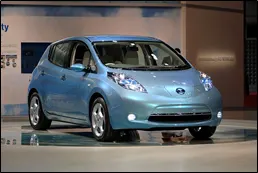
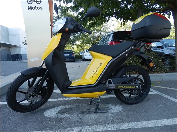
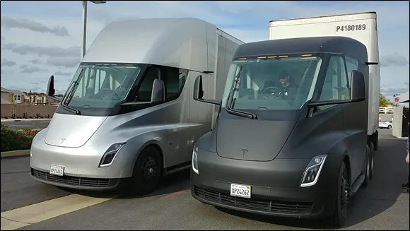
Commonly, the term EV is used to refer to an electric car. In the 21st century, EVs have seen a resurgence due to technological developments, and an increased focus on renewable energy and the potential reduction of transportation's impact on climate change and other environmental issues. Project Drawdown describes electric vehicles as one of the 100 best contemporary solutions for addressing climate change.

Government incentives to increase adoption were first introduced in the late-2000s, including in the United States and the European Union, leading to a growing market for the vehicles in the 2010s.And increasing consumer interest and awareness and structural incentives, such as those being built into the green recovery from the COVID-19 pandemic, is expected to greatly increase the electric vehicle market. As pre-COVID 2019 analysis, projected that Electric vehicles are expected to increase from 2% of global share in 2016 to 22% in 2030.Much of this market growth is expected in markets like North America and Europe; a 2020 literature review, suggested that growth in use of electric vehicles, especially electric personal vehicles, currently appears economically unlikely in developing economies.

• CALCULATION OF POWER REQUIRED:

FORCES ACTING ON VEHICLES:

Let us consider,

Mass of the vehicle = 500 Kg

Acceleration due to gravity = 9.81 m/s^2

Frontal area = 1.9 m^2

Drag coefficient = 0.19

Coefficient of rolling resistance = 0.015

Air density = 1.125 kg/m^3

Velocity of vehicle = 25 m/s

Radius of wheel = 0.38 m

No load speed N = 10000 rpm

1. Rolling Resistance Force:

`F_r = mu_r*m*g` where `mu_r` = coefficient of rolling resistance

m = mass of the vehicle

g = acceleration due to gravity

By substituting,

`F_r = 0.015*500*9.81 =73.575N`

2. Drag Force:

`F_d = 1/2 * rho*c_d*A*v^2` where `rho` = Air density

`c_d` = drag coefficient

A = Frontal area

v = velocity of vehicle

By substituting,

`F_d = 1/2 *1.125*0.19*1.9*25^2 = 126.91 N`

TOTAL TRACTIVE FORCE:

`F_(T) =F_r+F_d =73.575+126.91 =200.485N`

TORQUE CALCULATION:

`T = F_T*r` where `F_T` = Total tractive force

`r` = radius of tire

`T = 200.485*0.38 = 76.184 N-m`

POWER CALCULATION:

`P = T*omega` where T = torque in N-m

`omega` = angular velocity

`P = 76.18*(2*PI*10000/60) = 80kW`

BLOCKS USED FOR MODELLING:

VEHICLE BODY:

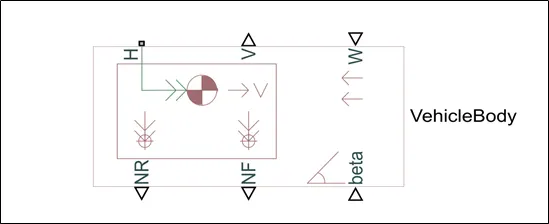
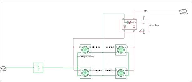
Represents a two-axle vehicle body in longitudinal motion. The block accounts for body mass, aerodynamic drag, road incline, and weight distribution between axles due to acceleration and road profile. The vehicle can have the same or a different number of wheels on each axle. Optionally include pitch and suspension dynamics or additional variable mass and inertia. The vehicle does not move vertically relative to the ground.

Connection H is the mechanical translational conserving port associated with the horizontal motion of the vehicle body. The resulting traction motion developed by tires should be connected to this port. Connections V, NF, and NR are physical signal output ports for vehicle velocity and front and rear normal wheel forces, respectively. Wheel forces are considered positive if acting downwards. Connections W and beta are physical signal input ports corresponding to headwind speed and road inclination angle, respectively. If variable mass is modeled, the physical signal input ports CG and M are exposed. CG accepts a two- element vector representing the x and y distance offsets from vehicle CG to additional load mass CG. M represents the additional mass. If both variable mass and pitch dynamics are included, the physical signal port J accepts the inertia of the additional mass about its own CG.

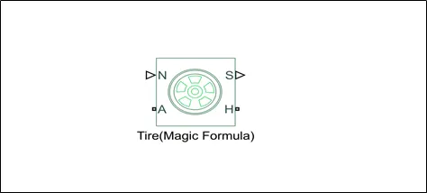
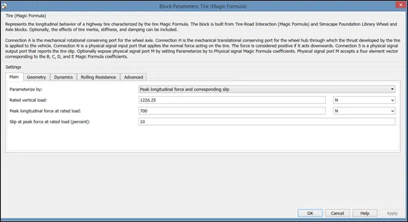
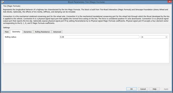
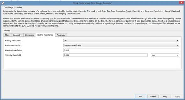
TIRE(MAGIC FORMULA):

Represents the longitudinal behavior of a highway tire characterized by the tire Magic Formula. The block is built from Tire-Road Interaction (Magic Formula) and Simscape Foundation Library Wheel and Axle blocks. Optionally, the effects of tire inertia, stiffness, and damping can be included.

Connection A is the mechanical rotational conserving port for the wheel axle. Connection H is the mechanical translational conserving port for the wheel hub through which the thrust developed by the tire is applied to the vehicle. Connection N is a physical signal input port that applies the normal force acting on the tire. The force is considered positive if it acts downwards. Connection S is a physical signal output port that reports the tire slip. Optionally expose physical signal port M by setting Parameterize by to Physical signal Magic Formula coefficients. Physical signal port M accepts a four element vector corresponding to the B, C, D, and E Magic Formula coefficients.

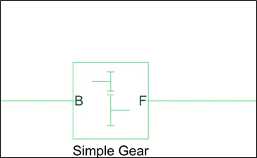
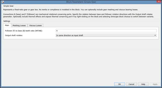
SIMPLE GEAR:

Represents a fixed-ratio gear or gear box. No inertia or compliance is modeled in this block. You can optionally include gear meshing and viscous bearing losses.Connections B (base) and F (follower) are mechanical rotational conserving ports. Specify the relation between base and follower rotation directions with the Output shaft rotates parameter. Optionally include thermal effects and expose thermal conserving port H by right-clicking on the block and selecting Simscape block choices to switch between variants.

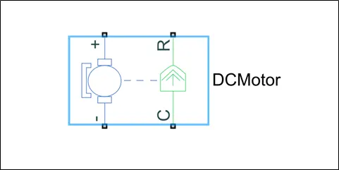
DC MOTOR:

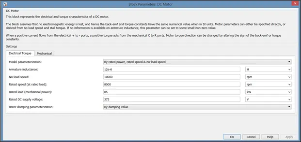
This block represents the electrical and torque characteristics of a DC motor.The block assumes that no electromagnetic energy is lost, and hence the back-emf and torque constants have the same numerical value when in SI units. Motor parameters can either be specified directly, or derived from no-load speed and stall torque. If no information is available on armature inductance, this parameter can be set to some small non-zero value.

When a positive current flows from the electrical + to - ports, a positive torque acts from the mechanical C to R ports. Motor torque direction can be changed by altering the sign of the back-emf or torque constants.

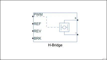
H-BRIDGE:

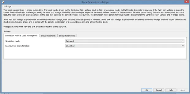
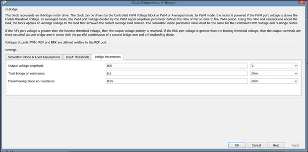
This block represents an H-bridge motor drive. The block can be driven by the Controlled PWM Voltage block in PWM or Averaged mode. In PWM mode, the motor is powered if the PWM port voltage is above the Enable threshold voltage. In Averaged mode, the PWM port voltage divided by the PWM signal amplitude parameter defines the ratio of the on-time to the PWM period. Using this ratio and assumptions about the load, the block applies an average voltage to the load that achieves the correct average load current. The Simulation mode parameter value must be the same for the Controlled PWM Voltage and H-Bridge blocks.

If the REV port voltage is greater than the Reverse threshold voltage, then the output voltage polarity is reversed. If the BRK port voltage is greater than the Braking threshold voltage, then the output terminals are short circuited via one bridge arm in series with the parallel combination of a second bridge arm and a freewheeling diode.Voltages at ports PWM, REV and BRK are defined relative to the REF port.

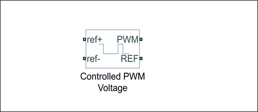
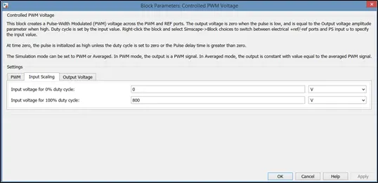
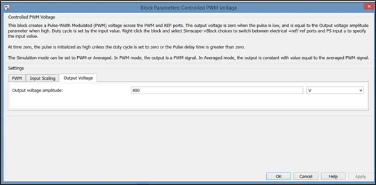
CONTROLLED PWM VOLTAGE:

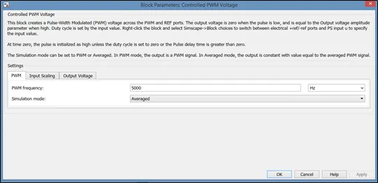
This block creates a Pulse-Width Modulated (PWM) voltage across the PWM and REF ports. The output voltage is zero when the pulse is low, and is equal to the Output voltage amplitude parameter when high. Duty cycle is set by the input value. Right-click the block and select Simscape->Block choices to switch between electrical +ref/-ref ports and PS input u to specify the input value.

At time zero, the pulse is initialized as high unless the duty cycle is set to zero or the Pulse delay time is greater than zero.

The Simulation mode can be set to PWM or Averaged. In PWM mode, the output is a PWM signal. In Averaged mode, the output is constant with value equal to the averaged PWM signal.

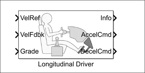
LONGITUDINAL DRIVER:

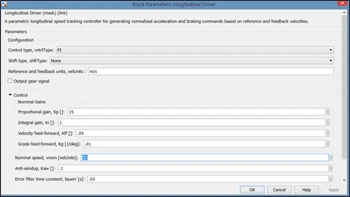
A parametric longitudinal speed tracking controller for generating normalized acceleration and braking commands based on reference and feedback velocities.

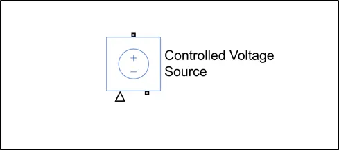
CONTROLLED VOLTAGE SOURCE:

The block represents an ideal voltage source that is powerful enough to maintain the specified voltage at its output regardless of the current passing through it. The output voltage is V = Vs, where Vs is the numerical value presented at the physical signal port.

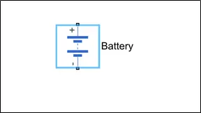
BATTERY:

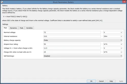
This block models a battery. If you select Infinite for the Battery charge capacity parameter, the block models the battery as a series internal resistance and a constant voltage source. If you select Finite for the Battery charge capacity parameter, the block models the battery as a series internal resistance plus a charge-dependent voltage source defined by:

V = Vnom*SOC/(1-beta*(1-SOC))

where SOC is the state of charge and Vnom is the nominal voltage. Coefficient beta is calculated to satisfy a user-defined data point [AH1,V1].

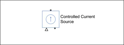
CONTROLLED CURRENT SOURCE:

The block represents an ideal current source that is powerful enough to maintain the specified current through it regardless of the voltage across it. The output current is I = Is, where Is is the numerical value presented at the physical signal port.

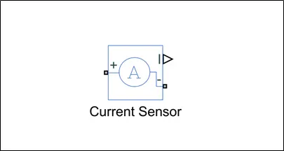
CURRENT SENSOR:

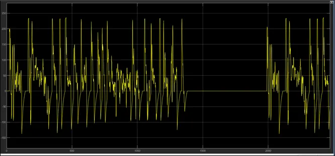
The block represents an ideal current sensor, that is, a device that converts current measured in any electrical branch into a physical signal proportional to the current.Connections + and - are conserving electrical ports through which the sensor is inserted into the circuit. Connection I is a physical signal port that outputs current value.

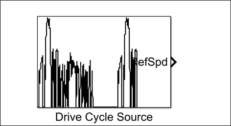
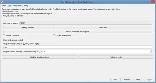
DRIVE CYCLE SOURCE:

A driving cycle is a series of data points representing the speed of a vehicle versus time.Driving cycles are produced by different countries and organizations to assess the performance of vehicles in various ways, as for instance fuel consumption, electric vehicle autonomy and polluting emissions.Fuel consumption and emission tests are performed on chassis dynamometers. Tailpipe emissions are collected and measured to indicate the performance of the vehicle.Another use for driving cycles is in vehicle simulations. More specifically, they are used in propulsion system simulations to predict performance of internal combustion engines, transmissions, electric drive systems, batteries, fuel cell systems, and similar components.Some driving cycles are derived theoretically, as it is preferred in the European Union, whereas others are direct measurements of a driving pattern deemed representative.

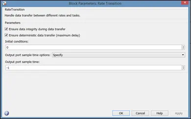
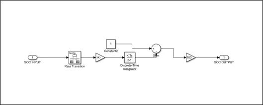
RATE TRANSITON:

Handle data transfer between different rates and tasks.

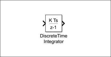
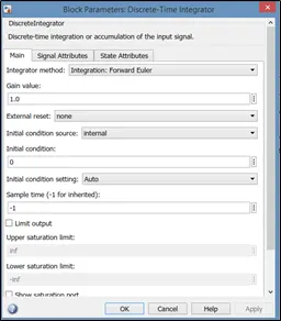
DISCRETE-TIME INTEGRATOR:

Discrete-time integration or accumulation of the input signal.

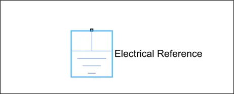
ELECTRICAL REFERENCE:

Electrical reference port. A model must contain at least one electrical reference port (electrical ground).

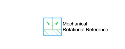
MECHANICAL ROTATIONAL REFERENCE:

This block represents a mechanical rotational reference point, that is, a frame or a ground. Use it to connect mechanical rotational ports that are rigidly affixed to the frame (ground).

CONSTANT:

Output the constant specified by the 'Constant value' parameter. If 'Constant value' is a vector and 'Interpret vector parameters as 1-D' is on, treat the constant value as a 1-D array. Otherwise, output a matrix with the same dimensions as the constant value.

SCOPE:

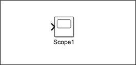
The Scope block can have multiple axes (one per port); all axes have a common time range with independent y-axes. The Scope allows you to adjust the amount of time and the range of input values displayed. You can move and resize the Scope window and you can modify the Scope's parameter values during the simulation.

SOLVER CONFIGURATION:

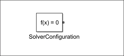
Defines solver settings to use for simulation.

MODEL PARAMETERS:

VEHICLE BODY:

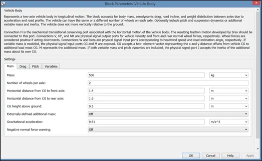
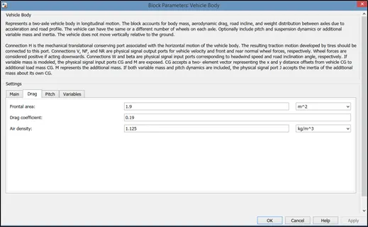
We have consider the mass of the vehicle as 500Kg and number of wheels per axle as two , drag coefficient as 0.19 which is used to calculate the drag force.

TIRE(MAGIC FORMULA):

SIMPLE GEAR:

DC MOTOR:

H-BRIDGE:

CONTROLLED PWM VOLTAGE:

LONGITUDINAL DRIVER:

BATTERY:

DRIVE CYCLE SOURCE:

RATE TRANSITION:

DISCRETE TIME INTEGRATOR:

MECHANICAL SUBSYSTEM:

STATE OF CHARGE SUBSYSTEM:

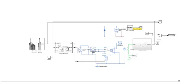
MATLAB MODEL:

• RESULTS:

VELOCITY SCOPE:

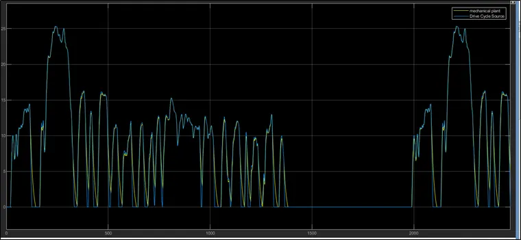
The blue plot represent the drive cycle source and yellow plot represents the actual velocity plot and the designed model is covering around 5.131km distance.

SOC SCOPE:

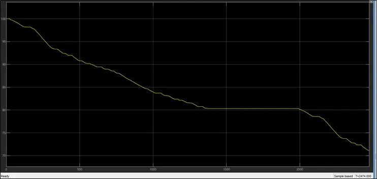
State of charge is 100% at the beginning of simulation and after simulation the state of charge is around 72%

CURRENT SENSOR:

VOLTAGE SENSOR:

• CONCLUSION:

We have created a MATLAB model of electric car which uses a battery and a DC motor by using powertrain blockset and drive cycle source as input to the model and we got a plot which is nearly exact to the given drive cycle source and designed model is performing well.