Final Project: Design of an Electric Vehicle

AIM: To design MATLAB model of electric car which uses a battery and a DC motor.

BLOCK DIAGRAM:

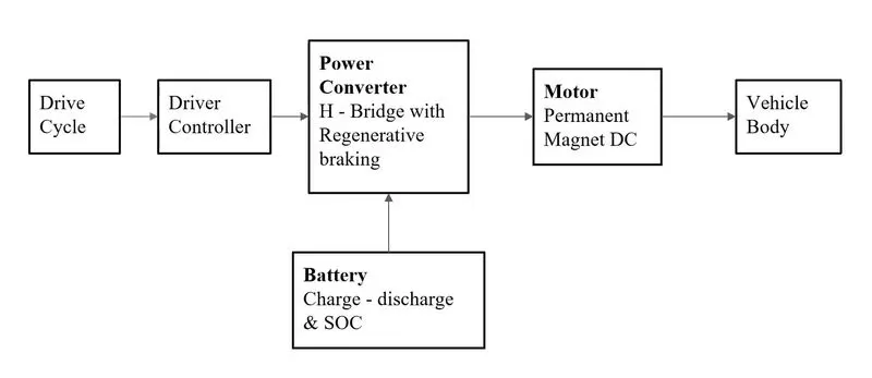
The following block diagram shows the main components used to design the electric car model.

The following diagram shows the full model view of electric vehicle model:

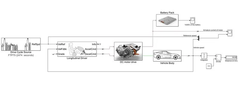
• Drive cycle source enables to choose various standard drive cycles or any random drive cycle (created by us) which acts as reference speed for the vehicle.
• Longitudinal driver acts like controller, which compares actual speed with reference speed and tries to reduce the error between them.
• Motor drive comprises of controller and DC motor where controller develops required voltage to the motor based on the commands given by the longitudinal driver and motor develops torque which propules the vehicle at required speed in either foward or reverse direction.
• Battery either discharges or charges according to the magnitude and polarity of the armature current of the DC motor.

Now, let us look into the every subsystems and blocks of the designed electric vehicle model one by one.

1). DRIVE CYCLE SOURCE:

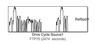
• Generates a standard or user-specified longitudinal drive cycle. The block output is the vehicle longitudinal speed. You can import drive cycles from:

1. Predefined sources
2. Workspace variables, including arrays and time series objects
3. mat, xls, xlsx, or txt files

• Use the fault tracking parameters to identify drive cycle faults within specified speed and time tolerances.

2). LONGITUDINAL DRIVER BLOCK:

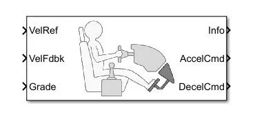
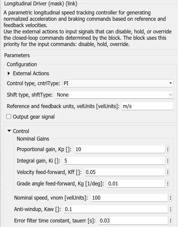
The Longitudinal Driver block implements a longitudinal speed-tracking controller. Based on reference and feedback velocities, the block generates normalized acceleration and braking commands that can vary from 0 through 1. You can use the block to model the dynamic response of a driver or to generate the commands necessary to track a longitudinal drive cycle.

Input ports:

• VelRef: Reference vehicle velocity (m/sec).
• VelFdbk: Longitudinal vehicle velocity (m/sec).
• Grade: Road grade angle in degrees (which is grounded i.e, grade angle = zero degrees).

Output ports:

• Info: Bus signal (here, it is terminated).
• AccelCmd: Commanded vehicle acceleration.
• DecelCmd: Commanded vehicle deceleration.

The following image shows parameters applied to the longitudinal driver block:

3). ELECTRIC DRIVE SUBSYSTEM:

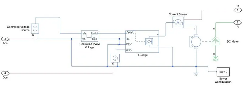
• The acceleration command which is output of 'longitudinal driver' block is applied to 'controlled PWM voltage' block through 'controlled voltage source' block.
• The deceleration command which is also output of 'longitudinal driver' block is applied to 'H-bridge' block through 'controlled voltage source' block.
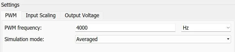
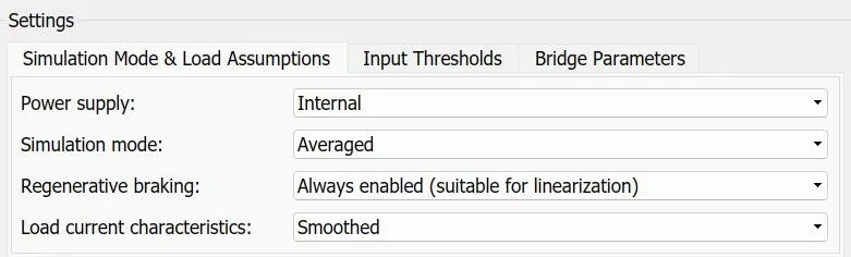
• Simulation mode is set to Averaged mode both in 'controlled PWM voltage' and 'H-bridge' blocks.
• Controlled PWM voltage delivers required PWM voltage to the H-brige block at pre-defined frequency.
• Here, H-bridge is powered using internal power supply.
• H-bride controls the magnitude and polarity of voltage applied to the DC motor terminals by which it can run the motor at required speed in required direction i.e, either in forward or reverse.
• The reference terminals of all blocks are connected to common electrical reference.

Controlled voltage source block:

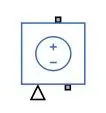
The block represents an ideal voltage source that is powerful enough to maintain the specified voltage at its output regardless of the current passing through it. The output voltage is V = Vs, where Vs is the numerical value presented at the physical signal port.

Controlled PWM voltage block:

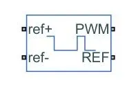
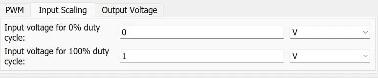
• This block creates a Pulse-Width Modulated (PWM) voltage across the PWM and REF ports. The output voltage is zero when the pulse is low, and is equal to the Output voltage amplitude parameter when high. Duty cycle is set by the input value. Right-click the block and select Simscape->Block choices to switch between electrical +ref/-ref ports and PS input u to specify the input value.
• At time zero, the pulse is initialized as high unless the duty cycle is set to zero or the Pulse delay time is greater than zero.
• The Simulation mode can be set to PWM or Averaged. In PWM mode, the output is a PWM signal. In Averaged mode, the output is constant with value equal to the averaged PWM signal.

Conserving ports:

• ref+: Positive terminal (Positive electrical reference voltage).
• ref- : Negative terminal (Negative electrical reference voltage).
• PWM:Pulse width modulated signal.
• REF: Floating zero volt reference.

The following images shows the parameters of controlled PWM voltage block:

H Bridge block:

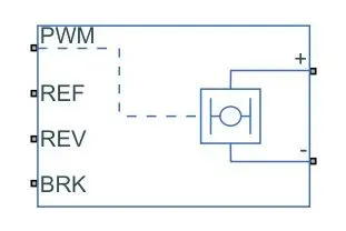
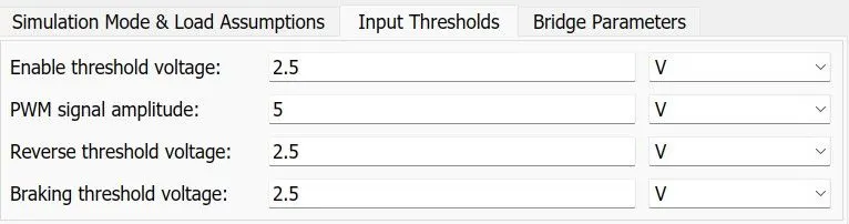
• This block represents an H-bridge motor drive. The block can be driven by the Controlled PWM Voltage block in PWM or Averaged mode. In PWM mode, the motor is powered if the PWM port voltage is above the Enable threshold voltage. In Averaged mode, the PWM port voltage divided by the PWM signal amplitude parameter defines the ratio of the on-time to the PWM period. Using this ratio and assumptions about the load, the block applies an average voltage to the load that achieves the correct average load current. The Simulation mode parameter value must be the same for the Controlled PWM Voltage and H-Bridge blocks.
• If the REV port voltage is greater than the Reverse threshold voltage, then the output voltage polarity is reversed. If the BRK port voltage is greater than the Braking threshold voltage, then the output terminals are short circuited via one bridge arm in series with the parallel combination of a second bridge arm and a freewheeling diode. Voltages at ports PWM, REV and BRK are defined relative to the REF port.
• If exposing the power supply connections, the block only supports PWM mode.

Conserving ports:

• PWM: Pulse Width Modulated signal (Electrical conserving port associated with the pulse-width modulated signal. The voltage is defined relative to the REF port).
• REF: Reference (Electrical conserving port associated with the floating zero volt reference)
• REV: Reverse (Electrical conserving port associated with the voltage that controls when to reverse the polarity of the H-Bridge block output. The voltage is defined relative to the REF port).
• BRK: Brake (Electrical conserving port associated with the voltage that controls when to short circuit the H-Bridge block output. The voltage is defined relative to the REF port).

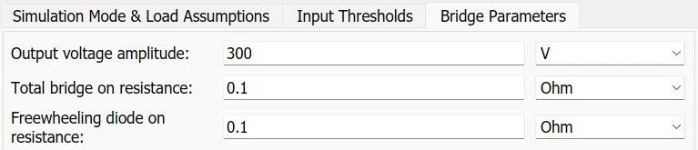
The following images shows the parameters that are defined for H-bridge block:

DC motor block:

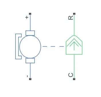
• This block represents the electrical and torque characteristics of a DC motor.
• The block assumes that no electromagnetic energy is lost, and hence the back-emf and torque constants have the same numerical value when in SI units. Motor parameters can either be specified directly, or derived from no-load speed and stall torque. If no information is available on armature inductance, this parameter can be set to some small non-zero value.
• When a positive current flows from the electrical + to - ports, a positive torque acts from the mechanical C to R ports. Motor torque direction can be changed by altering the sign of the back-emf or torque constants.

Conserving ports:

• +: DC motor's positive terminal.
• - : DC motor's negative terminal.
• R: Motor rotor.
• C:Motor case.

The following image shows the parameters which are defined for DC motor block:

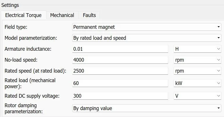
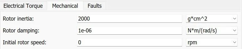
*No armature winding faults are enabled for DC motor block.

Solver configuration block:

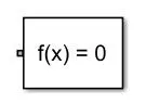
• Defines solver settings to use for simulation.
• Each physical network represented by a connected Simscape™ block diagram requires solver settings information for simulation. The Solver Configuration block specifies the solver parameters that your model needs before you can begin simulation.
• Each topologically distinct Simscape block diagram requires exactly one Solver Configuration block to be connected to it.

Current sensor block:

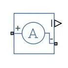
• The block represents an ideal current sensor, that is, a device that converts current measured in any electrical branch into a physical signal proportional to the current.
• Connections + and - are conserving electrical ports through which the sensor is inserted into the circuit. Connection I is a physical signal port that outputs current value.

Electrical reference block:

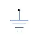
Electrical reference port. A model must contain at least one electrical reference port (electrical ground).

Rotational mechanical reference block:

This block represents a mechanical rotational reference point, that is, a frame or a ground. Use it to connect mechanical rotational ports that are rigidly affixed to the frame (ground).

4). BATTERY PACK SUBSYSTEM:

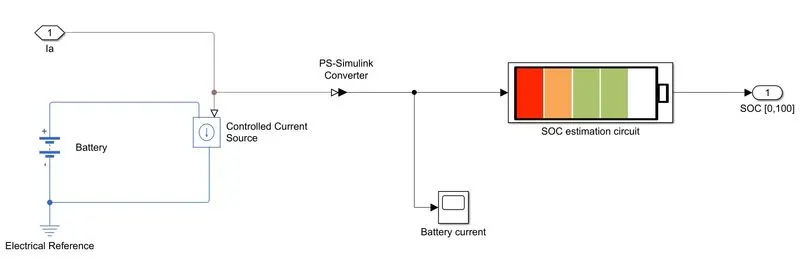
• Here, actually battery doesn't deliver current to the motor because H-bridge (which delivers the required current by the DC motor) is powered using internal power supply.
• But in practical, battery delivers required current by the motor. So, here circuit is designed in such a way that this battery is discharged according to the DC motor current.

Battery block:

This block models a battery. If you select Infinite for the Battery charge capacity parameter, the block models the battery as a series internal resistance and a constant voltage source. If you select Finite for the Battery charge capacity parameter, the block models the battery as a series internal resistance plus a charge-dependent voltage source defined by:

V = Vnom*SOC/(1-beta*(1-SOC))

where SOC is the state of charge and Vnom is the nominal voltage. Coefficient beta is calculated to satisfy a user-defined data point [AH1,V1].

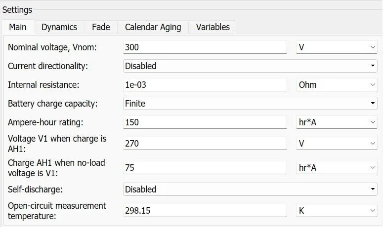
The following image shows the parameters of the battery which are defined in this model:

Controlled current source block:

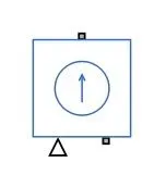
The block represents an ideal current source that is powerful enough to maintain the specified current through it regardless of the voltage across it. The output current is I = Is, where Is is the numerical value presented at the physical signal port.

PS - Simulink converter block:

• Converts the input Physical Signal to a Simulink output signal.
• The unit expression in 'Output signal unit' parameter must match or be commensurate with the unit of the Physical Signal and determines the conversion from the Physical Signal to the Simulink output signal.

5). SOC ESTIMATION CIRCUIT SUBSYSTEM:

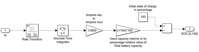
• State of Charge (SOC) is the level of charge of an electric battery relative to its capacity. For example, if SOC = 0%, the battery is empty and SOC = 100% then the battery is full.
• The SOC of the battery is estimated using the battery current which feeds current required by the DC motor.
• The rate transition block handles data transfer between different rates and tasks.
• The discrete time integrator integrates the battery current with respect to time (calculates area under the curve of current vs time) which obtains total charge (in Ampere seconds) delivered by the battery.
• The used capacity of the battery is converted to Ah (Ampere hour) from As (Ampere second) by multiplying the Ampere seconds with 1/3600 using gain block.
• The used capacity is converted to its percentage relative value of total battery capacity by dividing the used capacity with total battery capacity.
• SOC of the battery is obtained by substracting the used capacity in percentage value of total capacity from the initial state of charge i.e, 100% here.

Rate transition block:

• Handle data transfer between different rates and tasks.
• The Rate Transition block transfers data from the output of a block operating at one rate to the input of a block operating at a different rate. Use the block parameters to trade data integrity and deterministic transfer for faster response or lower memory requirements.

Gain block:

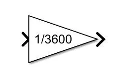
• Multiply input by constant.
• Element-wise gain (y = K.*u) or matrix gain (y = K*u or y = u*K).

Discrete time integrator block:

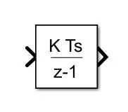
Perform discrete-time integration or accumulation of signal.

Constant block:

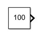
Output the constant specified by the 'Constant value' parameter. If 'Constant value' is a vector and 'Interpret vector parameters as 1-D' is on, treat the constant value as a 1-D array. Otherwise, output a matrix with the same dimensions as the constant value.

Sum block:

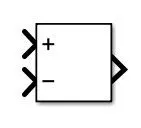
Add or subtract inputs depending upon the signs assigned to the input terminals.

6). VEHICLE BODY SUBSYSTEM:

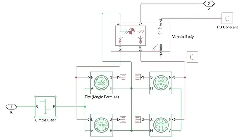
• Front tyres and rear tyres are connected to each other through their respective axles.
• Hubs of all the tyres are inter connected with horizontal motion port (H) of the vehicle body.
• Normal forces acting on the front and real axles are connected to the respective tyres.
• Slip (S) ports of all tyres are terminated using PS termination blocks.
• Head wind (W=0 m/sec) is applied through PS constant block.
• Grade angle (Beta=0 radians) is applied through the PS constant block.
• The base gear terminal (B) of the simple gear block is connected to the R terminal of the DC motor and its follower gear terminal (F)i s connected to the rear axle of the vehicle.

Vehicle body block:

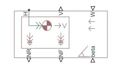
Represents a two-axle vehicle body in longitudinal motion. The block accounts for body mass, aerodynamic drag, road incline, and weight distribution between axles due to acceleration and road profile. The vehicle can have the same or a different number of wheels on each axle. Optionally include pitch and suspension dynamics or additional variable mass and inertia. The vehicle does not move vertically relative to the ground.

Input ports:

• W: Head wind speed in m/sec. (Here, we considered there is no head wind speed {W=0 is applied through physical constant})
• beta: road inclined angle in radians. (Here, beta is considered as zero radians applied through physical constant)

Output ports:

• V: Longitudinal velocity in m/sec.
• NF: Front axle normal force in Newtons.
• NR: Rear axle normal force in Newtons.

Conserving port:

• H: Horizontal motion.

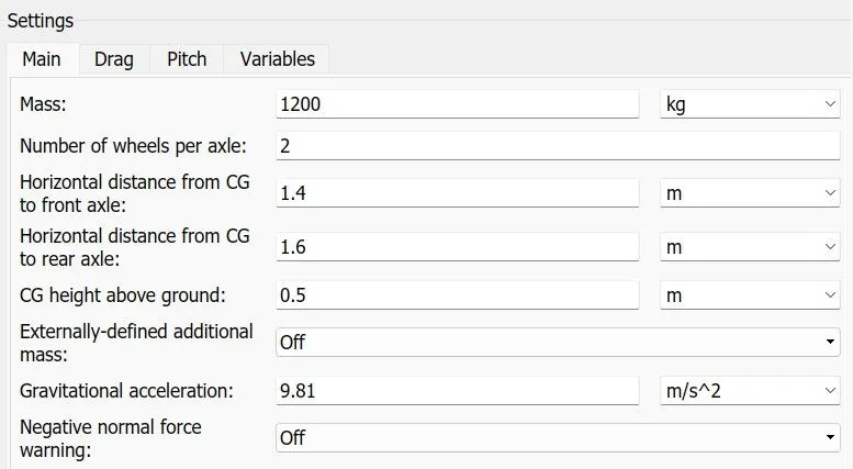
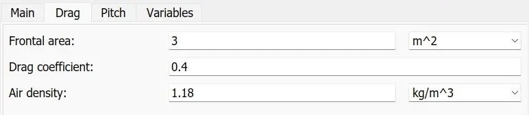
The following images shows the parameters and configurations applied in the vehicle body block:

*No modifications are made in 'pitch' and 'variables' section of settings.

Tyre (Magic formula) block:

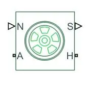
Represents the longitudinal behavior of a highway tire characterized by the tire Magic Formula. The block is built from Tire-Road Interaction (Magic Formula) and Simscape Foundation Library Wheel and Axle blocks. Optionally, the effects of tire inertia, stiffness, and damping can be included.

Input port:

• N: Normal force.

Output port:

• S: Slip.

Conserving ports:

• A: Axle.
• H: Hub.

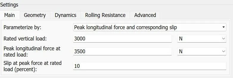
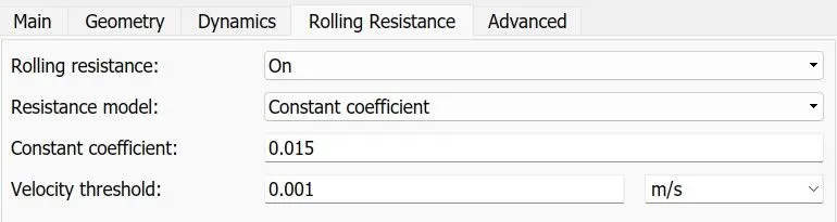
The following images shows the parameters implemented in the tyre block:

Simple gear block:

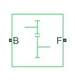
The Simple Gear block represents a gearbox that constrains the connected driveline axes of the base gear (B) and the follower gear (F) to corotate with a fixed ratio that you specify. You choose whether the follower axis rotates in the same or opposite direction as the base axis. If they rotate in the same direction, the angular velocity of the follower (`omega_F`) and the angular velocity of the base (`omega_B`) have the same sign. If they rotate in opposite directions, `omega_F` and `omega_B` have opposite signs.

Conserving ports:

• B: Base (Rotational mechanical conserving port associated with the base, or input, shaft).
• F: Follower (Rotational mechanical conserving port associated with the follower, or output, shaft).

The following image shows the parameters of the simple gear block:

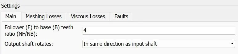
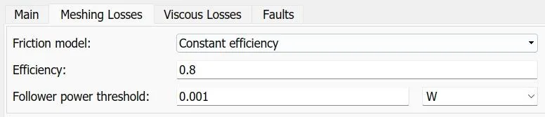
*Here, viscosous losses are considered as zero and no faults are enabled.

PS constant block:

This block creates a physical signal constant:

y = constant

The Constant parameter accepts both positive and negative values. The block output is a physical signal port.

PS terminator block:

Use this block to terminate physical signal outputs. Unconnected physical signal output ports do not generate warnings, but connection to a PS Terminator can be used to indicate that the signal was not inadvertently left unconnected.

7). CALCULATION OF DISTANCE TRAVELLED BY THE VEHICLE:

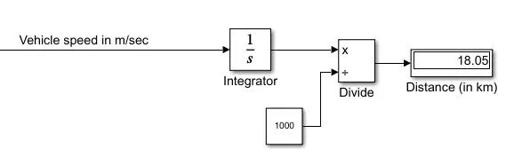
• Integrator integrates the velocity (in m/sec) with respect to time (In otherwords, it calculates area under the curve of velocity vs time) which obtains the distance travelled by the vehicle in meters.
• Distance travelled by the vehicle in kilometers (which is seen in 'display' block) is obtained by dividing the 'distance travelled in meters' with 1000 using 'divide' block.

RESULTS:

(i). The following image shows the armature current of DC motor plot in upper window and both reference speed & actual vehicle's speed in lower window.

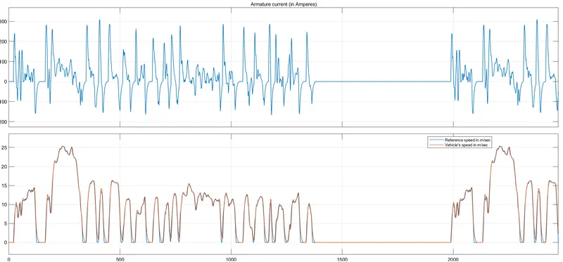
• Vehicle speed is almost identical to the reference speed at every instance of the simulation.
• Whenever the reference speed is approaching zero instantly, the vehicle taking more time to come to the rest due to of its inertia.
• From the armature current plot, we can observe that current becomes negative (i.e, motor acting as generator and delivering the current back to the battery) while the vehicle is decelerating. So we can conclude that the battery is in charging condition in this situation due to regenerative braking.
• Armature current reaches a peak value of 310A (around 2C rate) during discharging when maximum propulsion force required and of 170A (about 1.1C rate) during charging when large amount of braking force is required by the vehicle.

(ii).The following image shows the %SOC plot variation with respect to the time.

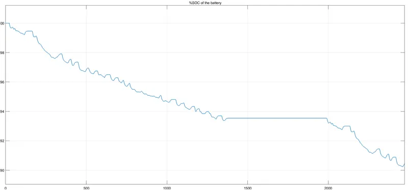
• Battery is in discharging mode (SOC is decreasing) whenever vehicle is accelerating or moving with constant speed.
• Battery is in charging mode (SOC is increasing) when the vehicle uses regenerative braking for deceleration.
• The battery is in neither in charging or discharging (i.e, SOC is not altered, remains constant) when the vehicle is in rest position from about 1370 to 1990 seconds of simulation.
• %SOC after driving through given FTP driving cycle is around 90.5% that means 9.5% of the battery is drained for travelling 18.05 kms.

CONCLUSIONS:

• Our designed vehicle slights unfollowed the reference speed while coming to the rest, as it took more time than the preferred due to of its inertia.
• The distance travelled by the vehicle is 18.05 kms when compared to its standard value of 17.7kms (which is FTP drive cycle's distance coverage), the difference is very small, so our vehicle almost follows the reference FTP drive cycle's speed which can be observed in the result plot.
• The vehicle travelled 18.05kms by consuming 9.5% of the battery, so it can travel around 190 kms on fully charged battery.