Final Project: Design of an Electric Vehicle

1)

An Electric Vehicles differ from a normal combustion vehicle based on the sorce of energy. Here despite of an engine an electric motor is used. This electric motor is controlled by a controller, and the controllers are in turn powered by rechargable batteries. A Battery Electric Vehicle (BEV), sometimes known as an All-Electric Vehicle (AEV), is a vehicle that runs solely on electricity. This type of electric vehicle does not have an internal combustion engine (ICE). Electricity is stored in a huge battery pack, which is charged by connecting to the power grid. The electric car is powered by one or more electric motors, which are powered by the battery pack.

The basic block diagram of an electric vehicle can be represented by:

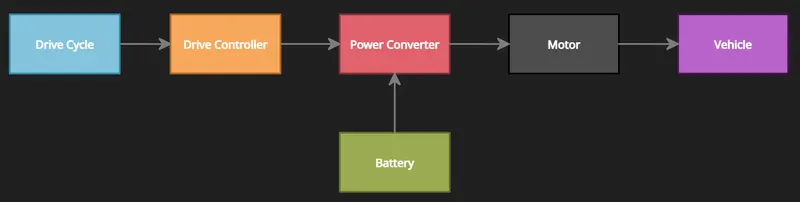
Our objective is to design an Electric Vehicle using MATLAB based on the above block diagram. Here drive cycle is the referance speed given into the controller or the driver and the Drive controller given specific acceleration or deceleration signals based on the referance to the Power converter (H-bridge) which is connected to the electric motor. The power converter controlls the speed of the electric motor based on the triggering or the pulses provided. The motor output is inturn connected to a mechanical system, a simple gear is used to transfer the mechanical power to the tyres.

Simulink Model:

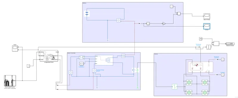
The simulink model depicts the block diagram shown above with a reference drive cycle, Drive controller as longitudinal drive, Motor controller with power converter H-bridge circuit, Battery system, And vehicle body which contains the mechanical parts.

Going forward with each subsystem, starting from the Vehicle:

SYSTEM LEVEL CONFIGURATIONS:

Vehicle:

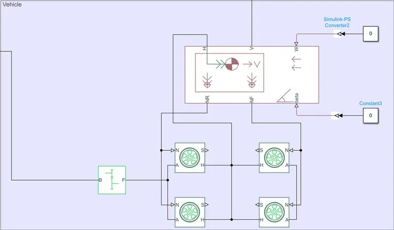
The vehicle subsystem consist of the vehicle body, Tyres and a simple gear.

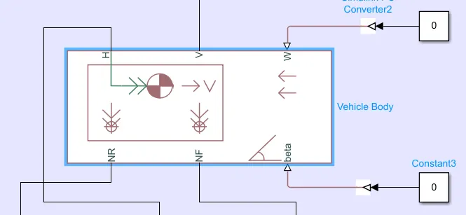
The Vehicle body consist of 6 ports which can be used to model various aspects of a vehicle.

Vehicle Body:

• H port - H stands for hub and is used to connect the hub to the wheels of the vehicle.
• V port - V stands for velocity, a physical signal and is used as and output which gives the vehicle velocity.
• W port - A physical signal input port which allows us to give the wind velocity experienced by the vehicle.
• NR port - A physical signal output port to connect the rear wheels.
• NF port - A physical signal output port to connect the front wheels.
• Beta - Input port to give inclination angle to the vehicle if any.

Model parameters include the vehicle topography like mass, frontal area etc...

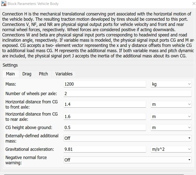
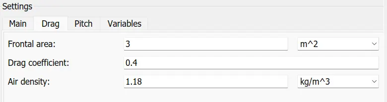
we can change all these model parameters according to our design from the block parameter dialog box of the vehicle body.

Tyre:

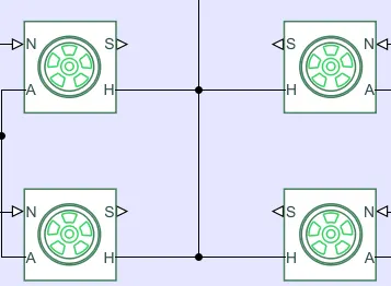
• Connection A - is the mechanical rotational conserving port for the wheel axle.
• Connection H - is the mechanical translational conserving port for the wheel hub through which the thrust developed by the tire is applied to the vehicle.
• Connection N - is a physical signal input port that applies the normal force acting on the tire. The force is considered positive if it acts downwards.
• Connection S - is a physical signal output port that reports the tire slip.

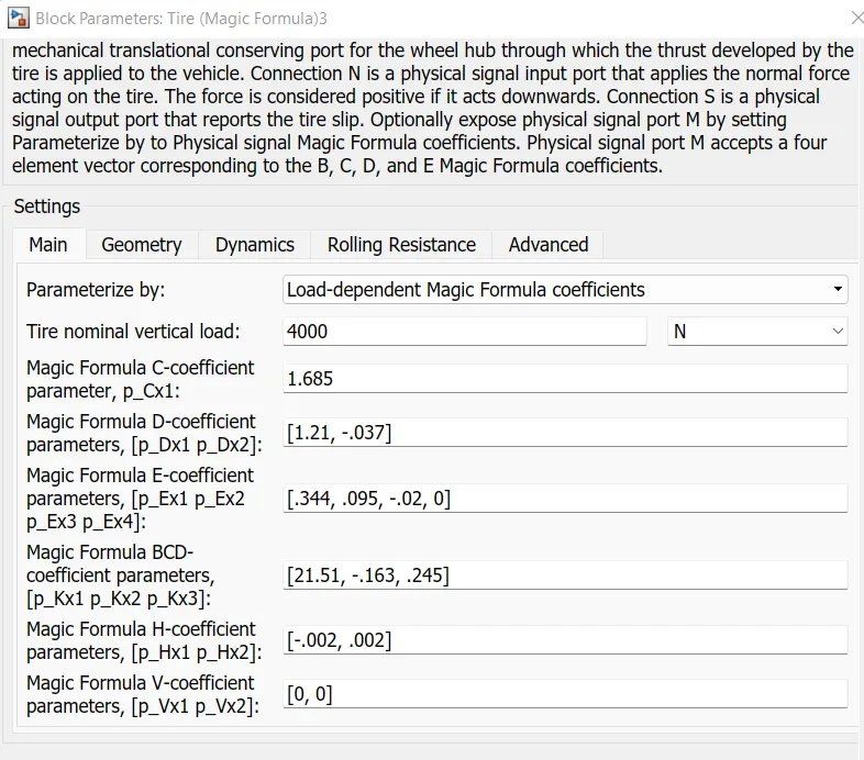
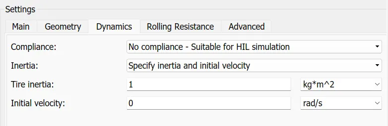
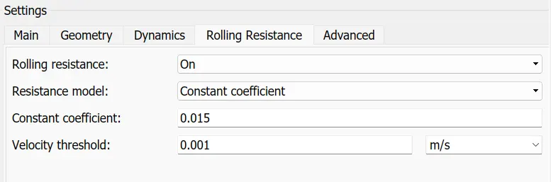
These are the model parameters of the tyre which we can chnage according to our design. We can assign the load, rolling radius, inertia, rolling resistance coefficient etc..

Simple gear:

Simple gear represents the gear box of the vehicle. It has two connections, 1 input and an output:

Connection B and Connection F stands for Base and Follower and are rotational conservating points.

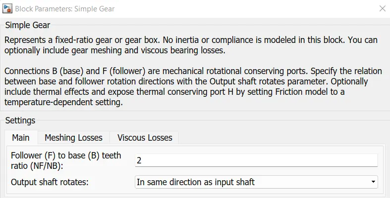
We can assign the teeth ratio between base and follower. And we can also decide whether the output shaft rotates in the same direction as of input or in the opposite direction. we can also provide mechanical losses within the block parameters.

Motor and Controller:

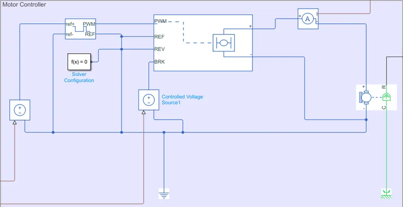
This block contains a DC motor of permananent magnet type, H-bridge, Controlled PWM voltage, Controlled voltage Source and a Current sensor.

DC-Motor:

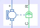
DC motors are easy to model and have very less model parameters considering a particular application. It has both electrical side and a mechanical side. When a positive curent flows through the electrical + and - ports, apositive torque will be developed in the emchanical C to R ports. C stands for casing (stable part) and R stands for rotor which produces the torque. The direction of torque can be changed bu altering the sign of the back emf or torque constants. The C port here is connected to mechanical rotaional referance and the R port is connected directly to the Base port of Simple gear block.

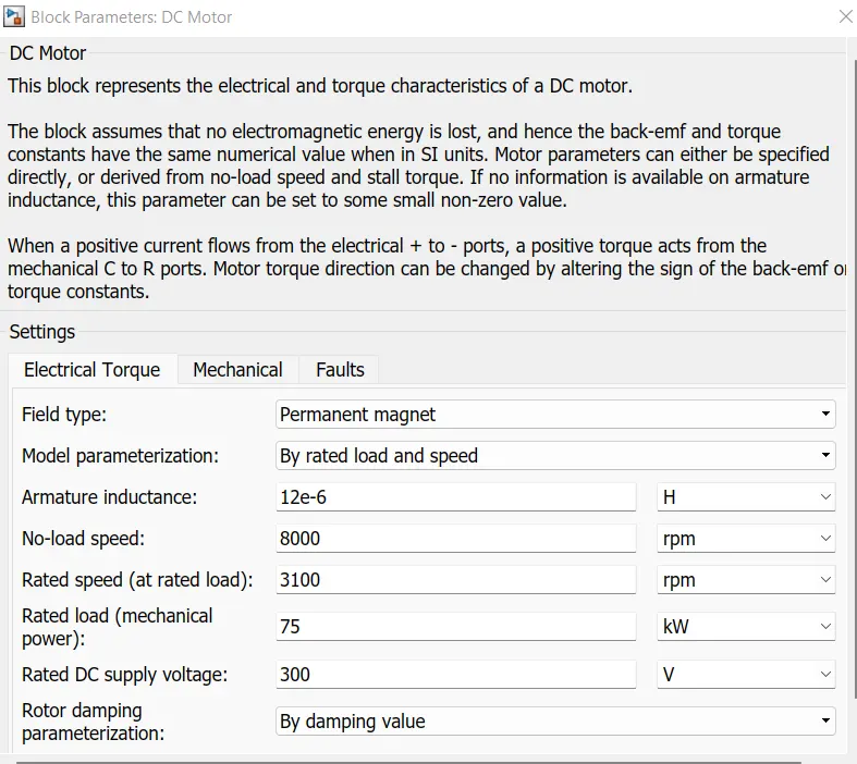
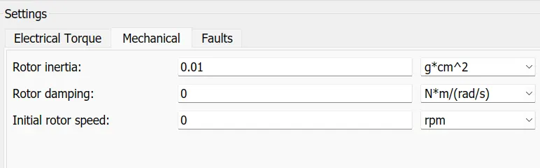
we can chnage the follwoing parameters from the motor block such as field type, Model parameterization which containd no load options also. Here following data are assigned for the specific model. Rotor inertia is also given.

H-Bridge:

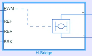
This represents the power converter block given in the block diagram. In an EV, a power converter is needed to provide power from the battery to the DC motor so that it can function properly at the required parameters. A controlled PWM block is used to drive the H-bridge motor drive in averaged mode. The ports of an H-bridge block are as follows:

• PWM - Pulse width modulation signals.
• REF - Reference
• REV - Reverse
• BRK - Brake

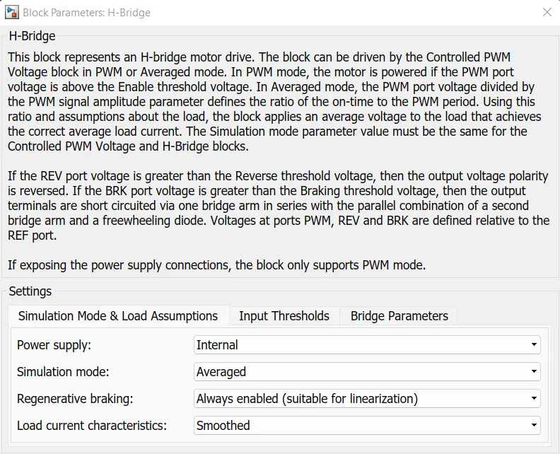
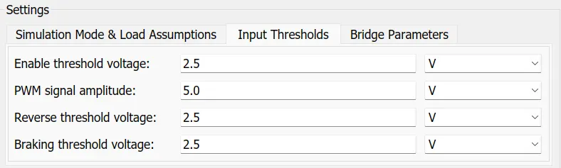
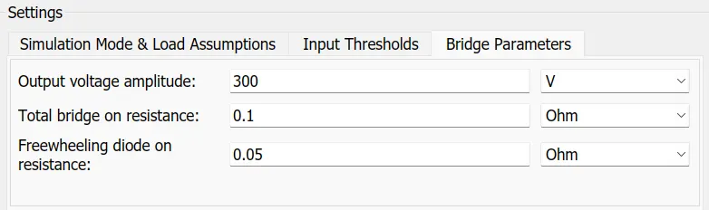
In Averaged mode, the PWM port voltage divided by the PWM signal amplitude parameter defines the ratio of the on-time to the PWM period. Using this ratio and assumptions about the load, the block applies an average voltage to the load that achieves the correct average load current. The Simulation mode parameter value must be the same for the Controlled PWM Voltage and H-Bridge blocks. If the REV port voltage is greater than the Reverse threshold voltage, then the output voltage polarity is reversed. If the BRK port voltage is greater than the Braking threshold voltage, then the output terminals are short circuited via one bridge arm in series with the parallel combination of a second bridge arm and a freewheeling diode. Voltages at ports PWM, REV and BRK are defined relative to the REF port.

Here the simulation is kept in averaged mode sisnce it requires less time to simulate and the output voltage is set to 300V in the bridge parameter.

Controlled PWM Voltage:

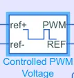
This block drives the H-bridge motor drive. The pulse created by the block solely depends on the duty cycle which is the ratio of on time to the time taken for 1 cycle.

Duty cycle = Ton/(Ton+Toff)

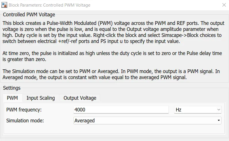
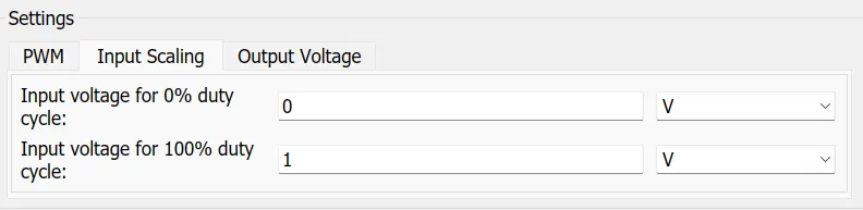
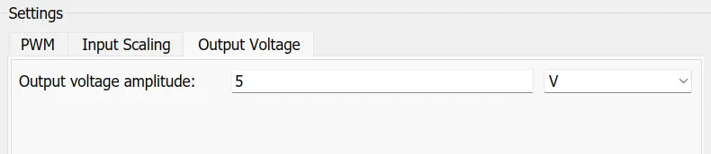
Here all the parameters are set to the default value. And simulation mode is switched to averaged as same as that of H-bridge.

Controlled Voltage Source:

The block provides the necessary voltage that is required for maintaining the voltage at the output regardless of the current that passs through it. We have used two such blocks, one for the acceleration and another for braking/deceleration.

Current Sensor:

The block represents an ideal current sensor, that is, a device that converts current measured in any electrical branch into a physical signal proportional to the current. Connections + and - are conserving electrical ports through which the sensor is inserted into the circuit. Connection I is a physical signal port that outputs current value.

Solver Configuration:

This block defines the solver settings to be used for the simulation.

Electrical Reference:

This block is known as the Electrical reference port. A model must contain at least one electrical reference port or electrical ground.

Mechanical Rotational Reference:

This block represents a mechanical rotational reference point, that is, a frame or a ground. Use it to connect mechanical rotational ports that are rigidly affixed to the frame (ground).

Battery Subsystem:

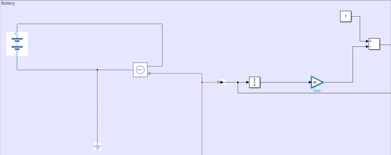
The subsystem is the only source of the vehicle. It powers the motor through the bridge circuit.

Battery:

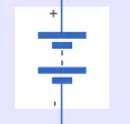
This block models a battery. It stores the energy inorder to drive the EV.

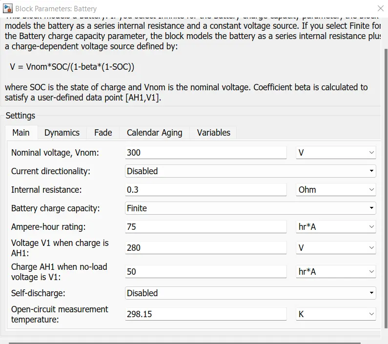
If we select Infinite for the Battery charge capacity parameter, the block models the battery as a series internal resistance and a constant voltage source. If we select Finite for the Battery charge capacity parameter, the block models the battery as a series internal resistance plus a charge-dependent voltage source defined by:

V = Vnom*SOC/(1-beta*(1-SOC))

where SOC is the state of charge and Vnom is the nominal voltage. Coefficient beta is calculated to satisfy a user-defined data point [AH1,V1].

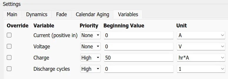
Here the finite mode selected and the nominal voltage is set to 300V. And internal resistance as 0.3 ohms. Other parameters are taken as default values.

Controlled Current Source:

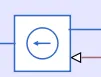
The block represents an ideal current source that is powerful enough to maintain the specified current through it regardless of the voltage across it. The output current is I = Is, where Is is the numerical value presented at the physical signal port.

SOC Estimation:

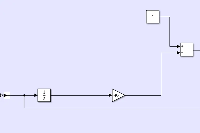
To measure the State of Charge (SOC) of the battery the following subsystem is used. Here the current signal from the H-bridge block or the current to the battery is integrated using an integrator block and multiplied with a defined gain. Then it is subtracted from 1 to get the SOC for the specific instance.

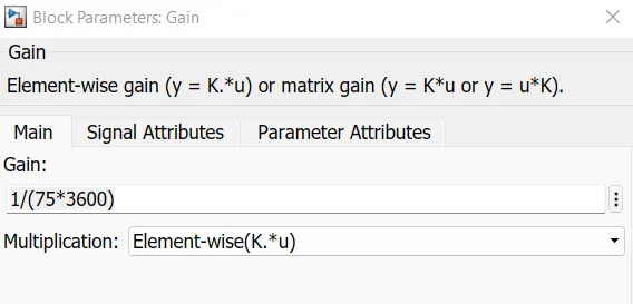
This shows the gain value defined for the SOC estimation.

Longitudinal Driver:

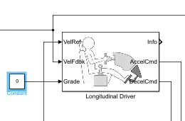
The longitudinal Driver block implements a longitudinal speed-tracking controller. The block generates normalized acceleration and braking commands ranging from 0 to 1 from the referance velocity of drive cycle and the feedback velocity from the vehicle. We can use the model to deliver dynamic response of a driver or to generate the commands necessary to track a longitudinal drive cycle.

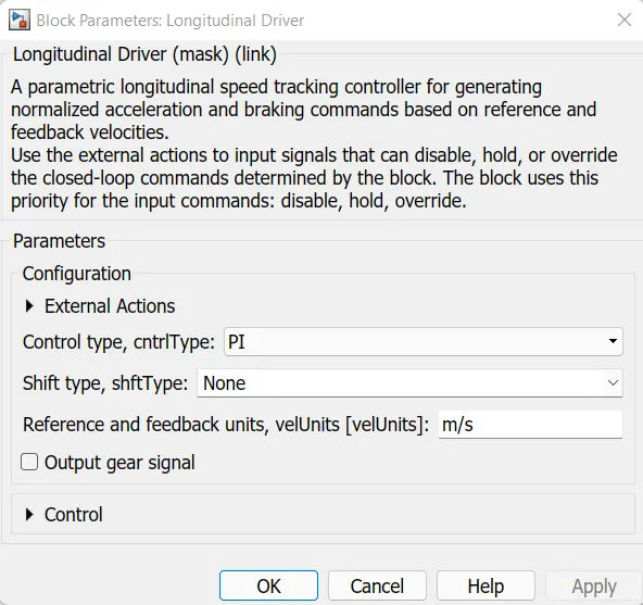
The control type varies from PI, Scheduled PI and predictive methods.

Drive Cycle:

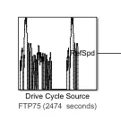
This block generates a standard or user-specified longitudinal drive cycle. The block output is the vehicle longitudinal speed and act as the referernce speed for the longitudinal driver. Here the FTP75 Drive cycle is used for the simulation.

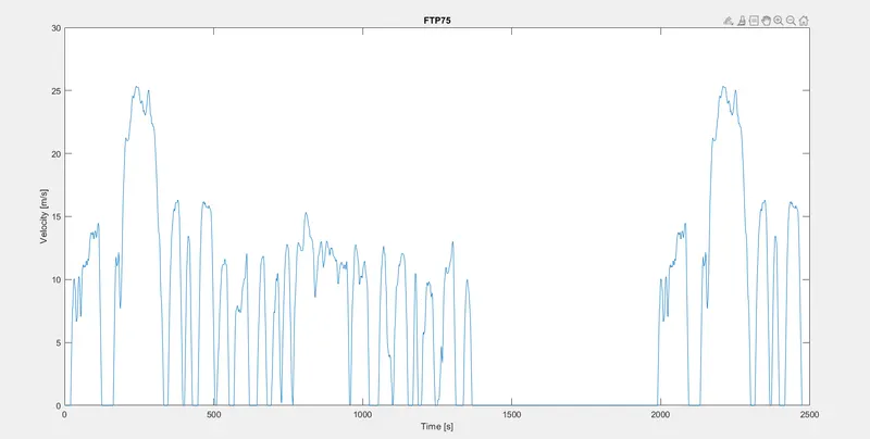
The reference speed can also be given in from a signal builder, or from excel sheet which can be connceted to the system using a multiport switch, from which the desired input can be chosen by given the constant value according to which switch it is connected.

RESULTS:

From the above simulation using Simulink, the following results were obtained.

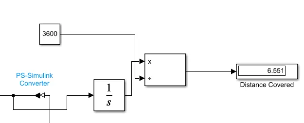
The Display block shows the distance travelled by the vehicle within the defined time period.

From the velocity of the vehicle and the input driving cycle the following results where obtained:

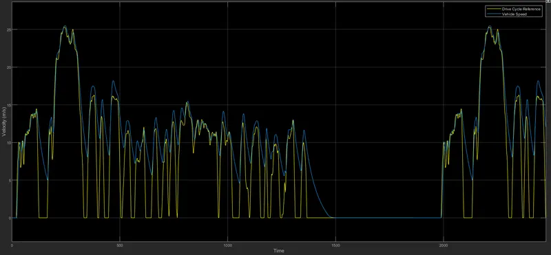
We can see that the vehicle has attained the velocity with respect to the reference drive cycle. Whenever during the deceleration the vehicle takes time to reach zero due to the inertia of the vehicle. Here exact overlapping is not scene due to some parameter changes. We can get promissing result by fine tuning the PI controller parameters of the longitudinal driver.

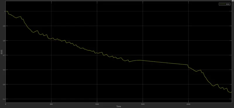
This graph shows the SOC of the battery through out the drive cycle. We can see some increase in soc when the vehicle is decelerating due to the regenerative braking. Throughout the journey we can see that the vehicle has used up around 55% of battery SOC and there will be around 45% SOC remaining.

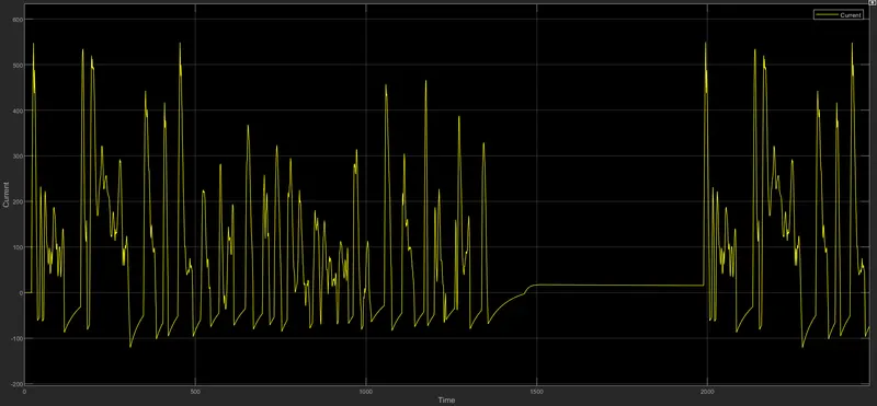
This graph shows the battery current throughout the drive cycle. Current goes negative during charging and we can see that the peak current when charging is much less that the peak current while discharging of the battery.

CONCLUSIONS:

The Matlab/Simulink Model of an electric car which uses a battery as the source and a DC motor has been succesfully implemented and simulated by using appropriate blocks from the Power Train blockset. From the simulated model the we came to the following conclusions:

From the Reference velocity or Duty Cycle versus actual velocity of the vehicle graph, we observed that the velocity of the vehicle model have approximately traced the FTP75 drive cycle given as reference. But when the speed drops to zero in the drive cycle the vehicle delays to reach zero due to the inertia of the vehicle. The tracing can be made perfect by further tuning the gains of the PI controller of the longitudinal driver, such that it corrects the acceleration and deceleration signals.

From the Battery SOC graph, we can see that almost 55% of the battery SOC has been utilized for completing the drive cycle. The spikes in the graph represents the regenerative braking during which the SOC graph will slightly increase. After completion of drive cycle we are almost left with 45% Battery SOC.

From the current graph we can see that the peak current value during normal driving is around 500A and during regerative braking this peak value is around 100A. Negative value of current indicates regenerative braking or charging of the battery. The peak discharging current will always be greater than the peak charging limit and the distance covered by the vehicle is around 6.5 Km throughout the drive cycle.