Final Project: Design of an Electric Vehicle

1.

Main Objective :

* To create a simulink model of an Electric Vehicle by using battery and motor modules

* To run the model and to check the performance of the model and its parameters

* To observe the results and to notedown

Here is the basic thing of an Electric vehicle and its construction and modeling

An electric vehicle (EV) is one that operates on an electric motor, instead of an internal-combustion engine that generates power by burning a mix of fuel and gases. Therefore, such as vehicle is seen as a possible replacement for current-generation automobile, in order to address the issue of rising pollution, global warming, depleting natural resources, etc. Though the concept of electric vehicles has been around for a long time, it has drawn a considerable amount of interest in the past decade amid a rising carbon footprint and other environmental impacts of fuel-based vehicles

Electric vehicles have low running costs as they have less moving parts for maintaining and also very environmentally friendly as they use little or no fossil fuels (petrol or diesel). While some EVs used lead acid or nickel metal hydride batteries, the standard for modern battery electric vehicles is now considered to be lithium ion batteries as they have a greater longevity and are excellent at retaining energy, with a self discharge rate of just 5% per month. Despite this improved efficiency, there are still challenges with these batteries as they can experience thermal runaway, which have, for example, caused fires or explosions in the Tesla model S, although efforts have been made to improve the safety of these batteries.

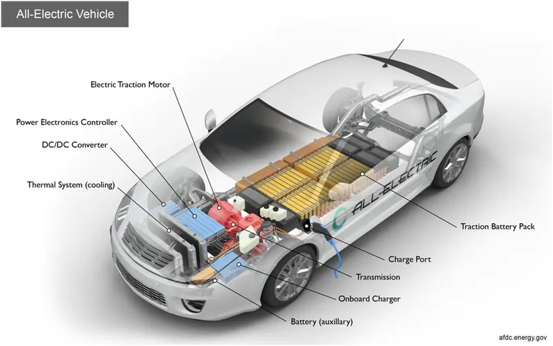
There are two main types of electric vehicles (EV); fully electric and plug-in hybrids:

Battery Electric Vehicles (BEV)

Compared to an internal combustion engine, battery powered electric vehicles have approximately 99% fewer moving parts that need maintenance.

Advantages of a BEV:

• Creates very little noise
• No exhaust, spark plugs, clutch or gears
• Doesn't burn fossil fuels, instead uses rechargeable batteries

BEVs can be charged at home overnight, providing enough range for average journeys. However, longer journeys or those that require a lot of hill climbs may mean that the fuel cells require charging before you reach your destination, although regenerative braking or driving downhill can help mitigate against this by charging the battery packs.

The typical charging time for an electric car can range from 30 minutes and up to more than 12 hours. This all depends on the speed of the charging station and the size of the battery.

In the real world, range is one of the biggest concerns for electric vehicles, but is something that is being addressed by industry.

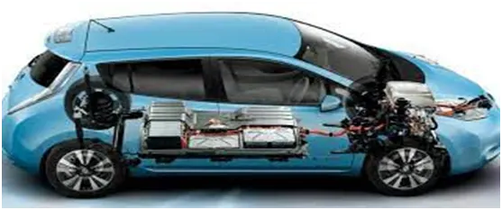
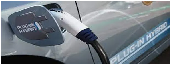
Plug-in Hybrid Electric Vehicles (PHEV)

Rather than relying solely on an electric motor, hybrid electric vehicles offer a mixture of battery and petrol (or diesel) power. This makes them better for travelling long distances as you can switch to traditional fuels rather than having to find charge points to top up the battery.

Of course, the same disadvantages that apply to combustion engine vehicles also apply to PHEVs, such as the need for more maintenance, engine noise, emissions and the cost of petrol. PHEVs also have smaller battery packs, which means a reduced range.

Motors :

The Specific Types of EV Motors. Beyond the categories of electric motors mentioned earlier, there are three types most often used in EVs: brushless asynchronous induction motors, brushed externally excited synchronous motors, and brushless permanent magnet synchronous motors

BLDC motors are suitable for high power density design approach. The BLDC motors are the most preferred motors for the electric vehicle application due to its traction characteristics. You can learn more about BLDC motors by comparing it with normal brushed motor.

A typical motor will be in the 20,000-watt to 30,000-watt range. A typical controller will be in the 40,000-watt to 60,000-watt range (for example, a 96-volt controller will deliver a maximum of 400 or 600 amps)

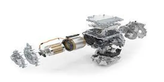
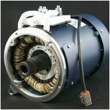
below we can observe the assembeled motor part.

Battery :

Lithium-ion batteries

Most plug-in hybrids and all-electric vehicles use lithium-ion batteries like these. Energy storage systems, usually batteries, are essential for hybrid electric vehicles (HEVs), plug-in hybrid electric vehicles (PHEVs), and all-electric vehicles (EVs).

Under current estimates, most EV batteries will last somewhere between 10-20 years before they need to be replaced

Lead-Acid Batteries

Lead-acid batteries can be designed to be high power and are inexpensive, safe, and reliable. However, low specific energy, poor cold-temperature performance, and short calendar and cycle life impede their use. Advanced high-power lead-acid batteries are being developed, but these batteries are only used in commercially available electric-drive vehicles for ancillary loads.

Ultra capacitors

Ultra capacitors store energy in a polarized liquid between an electrode and an electrolyte. Energy storage capacity increases as the liquid's surface area increases. Ultra capacitors can provide vehicles additional power during acceleration and hill climbing and help recover braking energy. They may also be useful as secondary energy-storage devices in electric-drive vehicles because they help electrochemical batteries level load power.

Recycling Batteries

Electric-drive vehicles are relatively new to the U.S. auto market, so only a small number of them have approached the end of their useful lives. As a result, few post-consumer batteries from electric-drive vehicles are available, thus limiting the extent of battery-recycling infrastructure. As electric-drive vehicles become increasingly common, the battery-recycling market may expand.

Widespread battery recycling would keep hazardous materials from entering the waste stream, both at the end of a battery's useful life and during its production. Work is now under way to develop battery-recycling processes that minimize the life-cycle impacts of using lithium-ion and other kinds of batteries in vehicles.

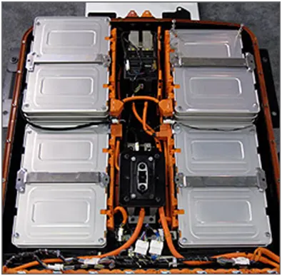
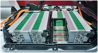
Compared to liquid fuels, most current battery technologies have much lower specific energy, and this often impacts the maximum all-electric range of the vehicles. The most common battery type in modern electric vehicles are lithium-ion and lithium polymer, because of their high energy density compared to their weight.

ON-Board Charger:

At the heart of any electric (EV) or plug-in hybrid (HEV) vehicle lays the high-voltage (200 to 450 VDC) battery and its associated charging system. The on-board charger (OBC) provides the means to recharge the battery from the AC mains either at home or from outlets found in private or public charging stations. From a 3.6 kW single-phase to a 22 kW three-phase high-power converter, today's (OBCs) On-Board Chargers must have the highest possible efficiency and reliability to ensure rapid charging times as well as meet the limited space and weight requirements.

The primary role of an on-board charger (OBC) is to manage the flow of electricity from the grid to the battery. This means that the OBC must comply with the requirements of the grid in locations where it will be used

To begin with, an onboard charger is simply a charger that is mounted in the vehicle itself and only requires a wire and plug to charge the vehicle. The onboard charger does convert AC power, which is available virtually everywhere, into the much-needed DC power required to charge the battery

While the onboard charger has to condition (convert to high-voltage DC) power from the off-board AC charger before supplying it to the battery management system (BMS), the off-board DC charger works without an onboard charger and interfaces directly with the BMS

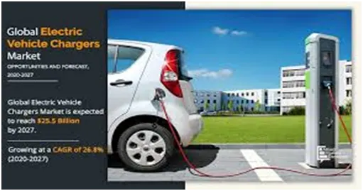
the above image represents the basic outdoor vehicle charging point (Road-side poiny)

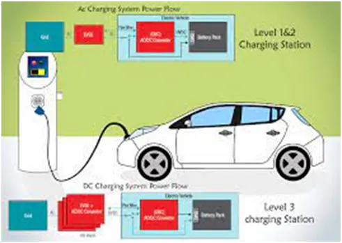
EV control unit (EV-ECU) is the control unit to manage the electric vehicle operations. EV Control Unit (EV-ECU) is a controller to control vehicle dynamics based on information from Inverter, BMU and Charger etc.

Power is converted from the DC battery to AC for the electric motor. The accelerator pedal sends a signal to the controller which adjusts the vehicle's speed by changing the frequency of the AC power from the inverter to the motor. The motor connects and turns the wheels through a cog.

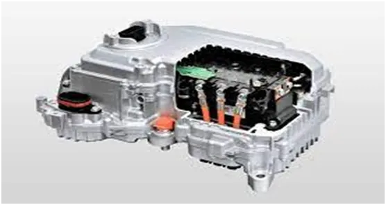
The power control unit for electric vehicles is an integrated control unit composed of a motor control unit, LDC, and VCU, and it controls and manages the overall operation of the vehicle including the driving condition of the vehicle.

1) Motor control unit
- Torque control for the vehicle’s drive motor
2) LDC: Low voltage DC-DC converter (low-voltage DC converter)
- Converts the high voltage battery’s high voltage to low voltage (DC 360V → DC 12V) to supply power to electrical components
3) VCU: Vehicle control unit (electric vehicle control unit)
- Control tower that oversees the operation of the electric vehicle

Block Diagram :

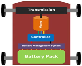
Now let’s see the basic block diagram of the electric vehicle (EV) system.

Here the main blocks of an Electric Vehicle are:

1. Battery
2. Motor controller part
3. Transmission system
4. Wheels

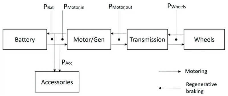
Here the duty cycle is given as an input to the system , according to the drive cycle the acceleration and the deceleration modes are performed. According to the duty cycle the power is fed from the battery source and according to the drive cycle the power is fed simultaneously to the motor terminals. According to the input voltage the motor operation is performed. As the motor runs the power generated in the motor block is transmitted to the transmission gear system and the transmission gear system is connected to the tire alignment. So as the motor rotates and the energy is transmitted to the tires through the transmission system the vehicle is moved either in forward direction or in reverse direction.

So, now let’s get in to the MATLAB modeling of the electric car

In MATLAB I had created an electric vehicle model (EV) by using the Battery, Motor, and some other transmission blocks. Here below I am attaching the figure of the EV model that I created in the SIMULINK.

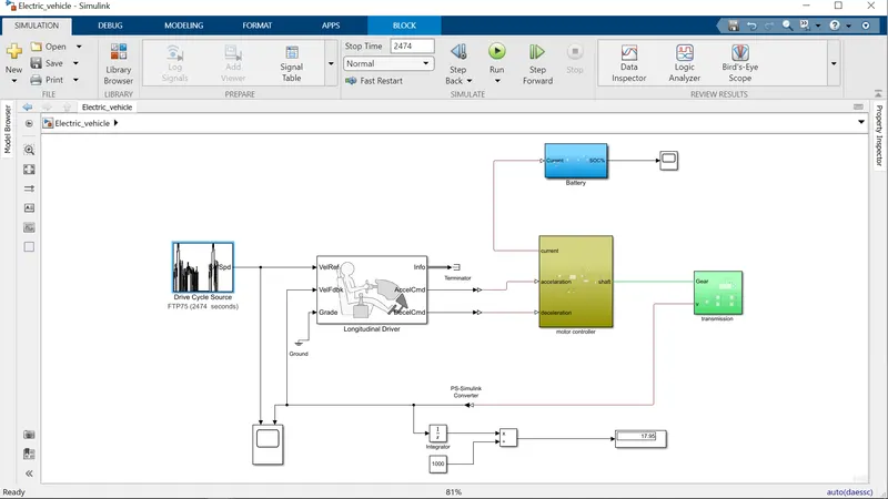
here i had built the model by using the different kind of blocks and the different kind of sub-systems in the SIMULINK which are explained in detail at below discreption about all the (Battery, motor controller & transmission) subsystems.

Detalied explanation of the model :

so. here lets go through step by step in the explanation of the model from the starting onwards.

1. Drive cycle :

here the drive cycle is taken as a input for the system with respective of the time and under the certain road and traffic conditions.

The Drive Cycle Source block generates a standard or user-specified longitudinal drive cycle. The block output is the specified vehicle longitudinal speed, which you can use to Predict the engine torque and fuel consumption that a vehicle requires to achieve desired speed and acceleration for a given gear shift reference.it also Produce realistic velocity and shift references for closed loop acceleration and braking commands for vehicle control and plant models. Study, tune, and optimize vehicle control, system performance, and system robustness over multiple drive cycles. this block identify the faults within tolerances specified by standardized tests. it has various types of cycles in this block

1. FTP75

2. Wide open throtal (WOT)

3. Work space and other options from where we can import the data

the below figure represents the drive cycle block :

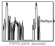
but in our model we had taken FTP75 drive cycle which is a basic and commonly used drive cycle for performance testing. and the time period of this drive cycle is 2474 sec. below i am attaching the image of the drive cycle that i had implemented in my model and its parameters.

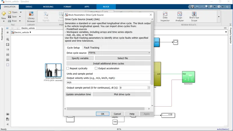
and by moving forward from this block if we observe i had connected my drive cycle block to the longitudinal driver block.

so, next lets see about this longitudinal driver block and its parameters.

2. Longitudinial driver :

this is a kind of assumption block with a driver operation with in the model. the Longitudinal Driver block implements a longitudinal speed-tracking controller. Based on reference and feedback velocities, the block generates normalized acceleration and braking commands that can vary from 0 through 1. we can utilize the block to model the dynamic response of a driver or to generate the commands necessary to track a longitudinal drive cycle. the below picture represents the basic block of logitudinial driver.

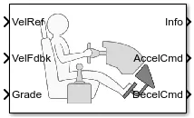
coming to the connections VELREF port is connected to the drive cycle block and VELFdbk port is connected to the feedback port from the vehicle body (V terminal). and the grade is connected to the ground block as the gradeability is not considered in this model. the INFO port is connected to the termonator block and the acceleration and deceleration command ports is connected to the respective ports of the motor control sub-system.

coming to the block parameters the control type is taken as PI. PI means proprtiona integral control with tracking wind-up and feed-forward gain. for the scheduled PI configuration the block used feed forward gains that are a function of vehicle velocity. and below i am attaching the image of the parameters considered for the following block

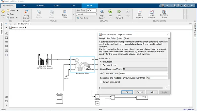
and after going forward from this block my next one is a Sub-system (motor control) and it is also connected with the longitudinal block.

lets explore the motor contro sub-system and its blocks and their parameters

3. Motor controller sub-system :

below i am attaching the image of the motor controller sub-system, in which we can observe each block used in it.

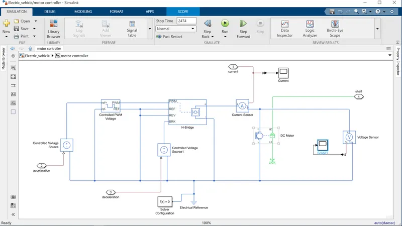
here if we observe the main blocks which acts as a heart of this sub-system are as follows :

i) H-bridge

ii) Controlled PWM voltage

iii) DC Motor

iv) Controlled voltage source

and the remaining blocks can be considered as a general blocks of the sub-system but those are also important blocks for the smooth and efficient operation, and those blocks are

v) Solver configuration

vi) Electric reference

vii) current sensor

viii) voltage sensor

ix) connection port

x) Scope

xi) mechanical rotational reference

so now lets see one-by-one block in detail and those block parameters.

i) H-bridge

The H-Bridge block represents an H-bridge motor driver. The block has the following two Simulation mode options: PWM — The H-Bridge block output is a controlled voltage that depends on the input signal at the PWM port.

If the input signal has a value greater than the Enable threshold voltage parameter value, the H-Bridge block output is on and has a value equal to the value of the Output voltage amplitude parameter. If it has a value less than the Enable threshold voltage parameter value, the block maintains the load circuit using one of the following three Freewheeling mode options:

* via one semiconductor switch and one freewheeling diode

* via two freewheeling diode

* via two semiconductor switches and one freewheeling diode

The first and third options are sometimes referred to as synchronous operation.

The signal at the REV port determines the polarity of the output. If the value of the signal at the REV port is less than the value of the Reverse threshold voltage parameter, the output has positive polarity; otherwise, it has negative polarity. the below image represents the basic block of H-bridge

now lets see the inside parameters of thos H-bridge according to our model. below i am attaching the image of this block parameters which i had considered.

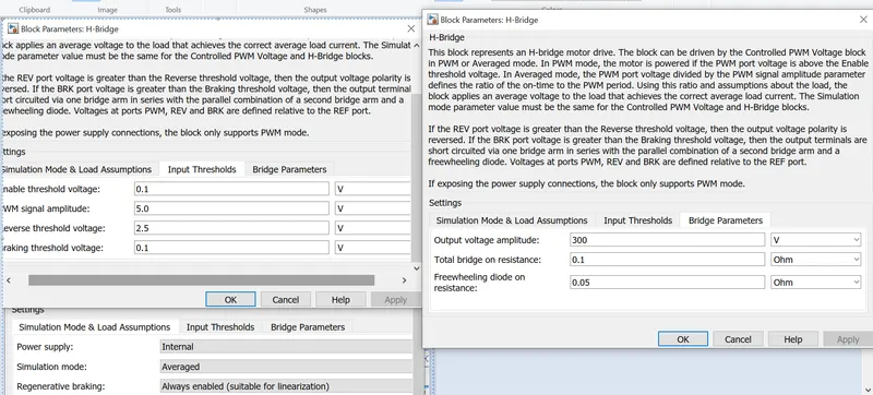
so, if we can observe the different kind of parameters in this H-bridge i.e., i)simulation mode and load assumptions, ii) input tresholds, iii) bridge parameters and according to our battery inputs and the motor specifications the input tresholds and the bridge parameters are modified

ii) Controlled PWM voltage :

The Controlled PWM Voltage block represents a pulse-width modulated (PWM) voltage source. You can model electrical or physical signal input ports by setting the Modeling option parameter to either:

If you set Modeling option to Electrical input ports, the demanded duty cycle is

At time zero, the pulse is initialized as high, unless the Pulse delay time parameter is greater than zero, or the demanded duty cycle is zero.

You can use parameters Pulse delay time and Pulse width offset to add a small turn-on delay and a small turn-off advance. This can be useful when fine-tuning switching times so as to minimize switching losses. the below picture represents the basic blockof controlled PWM voltage

the +ref is connected to the positive terminal of the controlled voltage source and the -ref port is connected to the negative port of the controlled voltage source and we can observe those connection in the above main image of the motor controlled Sub-system and now lets see the parameters which are considered in this block. below i am attaching the image of the considered parameters of the Controlled PWM voltage block

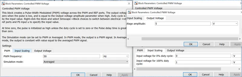
in the above if we observe we can modify the parameters of the followin i)PWM, ii) input scaling and iii) output voltage according to our specification of the model. and this is connected to the H-bridge as well.

and now lets move on to the another main block that is DC motor and its parameters.

iii) DC Motor :

DC motor driven by a constant input signal that approximates a pulse-width modulated signal and look at the current and rotational motion at the motor output.

it converts input electrical energy into mechanical motion

From the above definition, we can conclude that any electric motor that is operated using direct current or DC is called a DC motor. We will understand the DC motor construction and how a DC motor converts the supplied DC electrical energy into mechanical energy in the next few sections

magnetic field arises in the air gap when the field coil of the DC motor is energised. The created magnetic field is in the direction of the radii of the armature. The magnetic field enters the armature from the North pole side of the field coil and “exits” the armature from the field coil’s South pole side.

The conductors located on the other pole are subjected to a force of the same intensity but in the opposite direction. These two opposing forces create a torque that causes the motor armature to rotate. the below image represents the basic block of a DC motor in SIMULINK

the positive and negative terminals of the dc motor is connected to the positive and negative terminal of the H-bridge and the C terminal of the motor is connected to the mechanical rotational reference and the R port is connected to the Shaft of the transmission system. below i am attaching the image of the DC motor parameters which are considered.

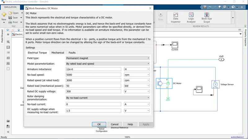
so if we see we can change the different kind of parameters like speed of the motot, rated supply voltage and the rated load and according to this the motor drive is operated.

and now lets see the controlled voltage source in this sub-system.

iv) Controlled voltage source :

The Controlled Voltage Source block converts a Simulink input signal into an equivalent voltage source. The generated voltage is driven by the input signal of the block. You can initialize the Controlled Voltage Source block with a specific AC or DC voltage.

If you want to start the simulation in steady state, the Simulink input must be connected to a signal that begins the simulation as a sinusoidal or DC waveform that corresponds to the initial values.

the controlled voltage source block represents an ideal voltage source that is powerful enough to maintain the specified voltage and its output regardless of the current flowing through the source.

the below image represents the basic block of an controlled volatage source

and this controlled voltage source is connected to H-bridge and the controlled PWM voltage blocks and we can observe thos connections in the main image of the motor controller sub-system and coming to its parameters there is no change in this block parameters and it is placed as it is in the system.

v) Solver configuration :

The Solver Configuration block specifies the solver parameters that your model needs before you can begin simulation. Each topologically distinct Simscape block diagram requires exactly one Solver Configuration block to be connected to it

Each physical network represented by a connected Simscape block diagram requires solver settings information for simulation. the below picture represents the basic block of solver configuration

with out this block the model is incomplete and it should be connected at anywhere in the physical system, in our model i had connected it at the ground terminal

vi) Electric reference:

The Electrical Reference block represents an electrical ground. Electrical conserving ports of all the blocks that are directly connected to ground must be connected to an Electrical Reference block. A model with electrical elements must contain at least one Electrical Reference block. this ground or electric reference block provides a return path to the electric circuit so it must be connected for the smooth operation and to avoid the faults. below image represents the basic block of electric reference.

vii) Current sensor:

The Current Sensor block represents an ideal current sensor, that is, a device that converts current measured in any electrical branch into a physical signal proportional to the current. this is also known as a type of ammeter which is used to mesure the value of current that is flowing in the circuit.

Use the + and - ports to connect the sensor in series with the other blocks in the branch where you want to measure the current. Port I outputs the measurement result as a physical signal. Use a ps simulink block to connect this port to Simulink blocks, such as Scope or Display. below picture represents the basic block of the current sensor

viii) Voltage sensor:

The Voltage Sensor block represents an ideal voltage sensor, that is, a device that converts voltage measured between two points of an electrical circuit into a physical signal proportional to the voltage. in electrical terminology it is also known as a voltmeter which is used to measure the voltage between the two terminals in the system or the corcuit.

Use the + and - ports to connect the sensor in parallel with the block (or several blocks) where you want to measure the voltage. Port V outputs the measurement result as a physical signal. Use a ps simulink converter block to connect this port to Simulink blocks, such as Scope or Display. below picture represents the basic block of the voltage sensor

ix) connection port:

The Connection Port block transfers a physical connection or signal across subsystem boundaries. Physical connections include Simscape conserving and physical signal connections, Simscape Multibody connections, and Vehicle Dynamics Blockset two-way connection ports, among others. we can connect subsystems and individual blocks by using this connection port.

A subsystem needs a Connection Port block for each physical connection line that crosses its boundary. You can manually place a Connection Port block inside a subsystem, or Simulink can automatically insert a Connection Port block when you create a subsystem within an existing network. below image represents the basic block of the connection port

x) Scope :

Scope, Floating Scope (Simulink Reference) The Scope block displays its input with respect to simulation time. The Scope block can have multiple axes (one per port); all axes have a common time range with independent y-axes. The Scope allows you to adjust the amount of time and the range of input values displayed.

we can connect multiple inputs to the scope so not only one output is displayed and we can also observe the other outputs also in scope. the below picture shows the basic block of the scope

xi) mechanical rotational reference :

The Mechanical Rotational Reference block represents a reference point, or frame, for all mechanical rotational ports. All rotational ports that are rigidly clamped to the frame (ground) must be connected to a Mechanical Rotational Reference block.

as we have a dc motor and it is also a mechanicalpart so the C port of the motor is connected to the mechanical rotational reference part. below image represents the basic block of the mechanical rotational reference

by here the motor controller sub-system explanation is ended and lets move for the next sub-system

our next sub-system is a Battery Sub-system and explore its parameters

4. Battery Sub-system :

below i am attaching the image of the battery sub-system which is in my model and lets look inti its perameters

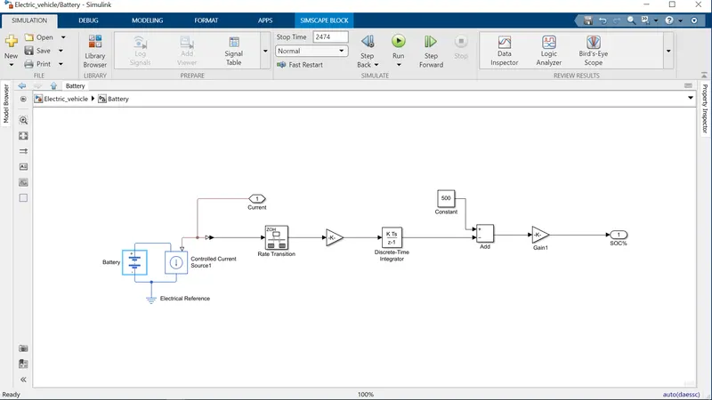
in this battery sub-system we have the following blocks. they are :

i) Battery

ii) controlled current source

iii) rate transition

iv) discrete time integrator

v) gain

vi) constant

vii) add

viii) connection port

so now lets see some of the main blocks in this sub-system

i) Battery

the battery play an important role in this system it is connected to the controlled current source and the electric reference in the system as it a kind of source it is charged and discharged according to the operation of the model and we can observe thd State of Charge (SOC) through scope and observe its value. the below figure represents the block of the battery

so, now lets see the perametersof the battery which is connected in this system and below i am attaching the image of the battery parameters which i have considered in this system

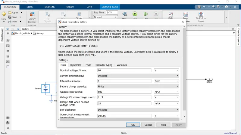
so, here i had taken the battery capacity as a finite and amp*hr rating i had considered is 500 as my motor rated load is 50kw

and this battery is connected to the controlled current source

ii) Controlled current source :

The Controlled Current Source block converts the Simulink input signal into an equivalent current source. The generated current is driven by the input signal of the block. The positive current direction is as shown by the arrow in the block icon

he Controlled Current Source block represents an ideal current source that is powerful enough to maintain the specified current through it regardless of the voltage across the source.

The output current is i = is where is = numerical value presented at the physical signal port.

The positive direction of the current flow is indicated by the arrow.

and coming to the parameters there is no need of change any kind of parameters in this block connect it as it is in the system

iii) Rate transition :

The Rate Transition block transfers data from the output of a block operating at one rate to the input of a block operating at a different rate. Use the block parameters to trade data integrity and deterministic transfer for faster response or lower memory requirements.

it is used to calculate the SOC curent in the model and the below image represents the block of rate transition

and the parameters of this block is attached below along with the parameters of the discrete time integrator parameters

iv) Discrete time integrator :

Use the Discrete-Time Integrator block in place of the Integrator block to create a purely discrete model. With the Discrete-Time Integrator block, you can: Define initial conditions on the block dialog box or as input to the block. Define an input gain (K) value. Output the block state. Define upper and lower limits on the integral. Reset the state with an additional reset input. below picture represents the block of the discrete time integrator

coming to the parameters there is no need to change any kind of parameters in this block. below i am ttaching the image of the considered parameters of discrete time integrator and the rate transition

v) Gain :

Gain (Using Simulink) The Gain block generates its output by multiplying its input by a specified gain factor. You can enter the gain as a numeric value, or as a variable or expression in the Gain parameter field. The input and gain can be a scalar, vector, or matrix.

The Multiplication parameter lets you specify whether to use element-by-element or matrix multiplication of the input by the gain.

the Gain block icon displays the value entered in the Gain parameter field if the block is large enough. If the gain is specified as a variable, the block displays the variable's name. below the image of the gain block is attached

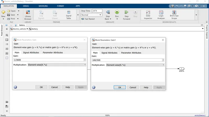
coming to the parameters we used this gain block two times in the model and now i am attaching the both gain blocks parameters in the below figure

vi) Constant :

The Constant block generates a real or complex constant value signal. Use this block to provide a constant signal input. The block generates scalar, vector, or matrix output, depending on: The dimensionality of the Constant value parameter. The setting of the Interpret vector parameters as 1-D parameter

The output of the block has the same dimensions and elements as the Constant value parameter. If you specify for this parameter a vector that you want the block to interpret as a vector, select the Interpret vector parameters as 1-D check box. Otherwise, if you specify a vector for the Constant value parameter, the block treats that vector as a matrix. below image represents the block of the constant

and now lets move on to the next subsystem i.e., transmission subsystem

5. Transmission sub-system :

below i am attaching the image of the transmission sub-system which is considered in my model and lets look inti its parameters one by one

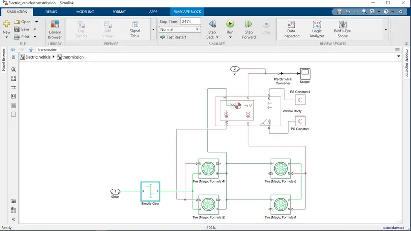
in the above picture if we observe the main blocks are

i) simple gear

ii) tire (magic formula)

iii) vehicle body

so lets see one by one block and its parameters

i) simple gear :

Represents a fixed-ratio gear or gear box. No inertia or compliance is modeled in this block. You can optionally include gear meshing and viscous bearing losses.

Connections B (base) and F (follower) are mechanical rotational conserving ports. Specify the relation between base and follower rotation directions with the Output shaft rotates parameter. Optionally include thermal effects and expose thermal conserving port H by setting Friction model to a temperature-dependent setting.

You choose whether the follower axis rotates in the same or opposite direction as the base axis. If they rotate in the same direction, the angular velocity of the follower, ω_F, and the angular velocity of the base, ω_B, have the same sign. If they rotate in opposite directions, ω_F and ω_B have opposite signs. You can easily add and remove backlash, faults, and thermal effects.

the below image represents the basic block of the simple gear

now lets get in the parameters which are considered in this block. below i am attaching the image of the considered parameters of this simple gear

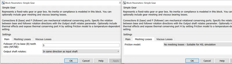
here we should conside main as an impotant parameter by which the gear opertion is changes and secondary is meshing losses.

now lets move to the next block that is tire and its parameters

ii) Tire (magic formula) :

The Tire (Magic Formula) block models a tire with longitudinal behavior given by the Magic Formula [1], an empirical equation based on four fitting coefficients. The block can model tire dynamics under constant or variable pavement conditions.

The longitudinal direction of the tire is the same as its direction of motion as it rolls on pavement. This block is a structural component based on the tire road interaction (magic formula) block.

To increase the fidelity of the tire model, you can specify properties such as tire compliance, inertia, and rolling resistance. However, these properties increase the complexity of the tire model and can slow down simulation. Consider ignoring tire compliance and inertia if simulating the model in real time or if preparing the model for hardware-in-the-loop (HIL) simulation. below image represents the tire basic block

lets see the parameters of this tire block in this model. below i am attaching the image of the considered parameters of this tire block in the system

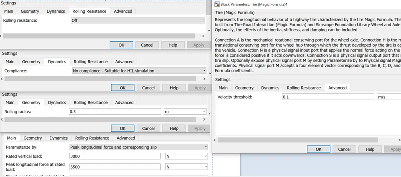
so if we observe we can see different kind of parameters of the tire and we can change those parameters according to the requirement of the model.

and the next block is vehicle body and its parameters

iii) Vehicle body :

The Vehicle Body block represents a two-axle vehicle body in longitudinal motion. The vehicle can have the same or a different number of wheels on each axle. For example, two wheels on the front axle and one wheel on the rear axle. The vehicle wheels are assumed identical in size. The vehicle can also have a center of gravity (CG) that is at or below the plane of travel.

The block accounts for body mass, aerodynamic drag, road incline, and weight distribution between axles due to acceleration and road profile. Optionally include pitch and suspension dynamics. The vehicle does not move vertically relative to the ground.

The block has an option to include an externally-defined mass and an externally-defined inertia. The mass, inertia, and center of gravity of the vehicle body can vary over the course of simulation in response to system changes.

he vehicle axles are parallel and form a plane. The longitudinal, x, direction lies in this plane and perpendicular to the axles. If the vehicle is traveling on an incline slope, β, the normal, z, direction is not parallel to gravity but is always perpendicular to the axle-longitudinal plane. below picture represents the basic block of the vehicle body

and we can observe the connections from the image of main sub-system of the transmission and now coming to the parameters below i am attaching the image of the considered parameters of the vehicle body block

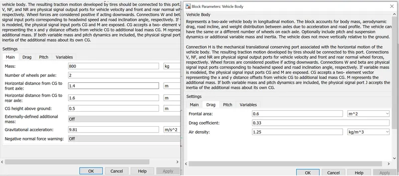
here we should change the value of mass in the main parameters and that value can be assumed and also we can see the drag parameters as well.

by now the explanation of the three subsystems which are there in my model are explored and explained and now lets get back to the main simulation page

here if we see the current port of the battery subsystem is connected to the corrent port of the motor controller and the shaft port of the motor controller is connected to the gear port of the transmission subsystem and v port of the transmission subsystem is connected to the scope for which the duty cycle is also connected by using ps simulink converter and to observe the distance travelled the display arrangement is also done at the below of the model with the help of the integrator and constant blocks.

here as we taken the drive cycle is FTP75 its duration is 2474sec so the run time of the model is also changed to 2474 sec. and now all the blocks and sub-systems are connected in this model and now lets run this model

and now lets see the discussion of the results which are obtained in the various scopes which are connected in the model

Scope Results : the obtained scope results are explained one-by-one at each constraint

Scope-1 :

the below scope is observed which is connected for the both duty cycle block and the velocity feedback from the transmission sub-system, and also inter connected to the longitudinal driver block.

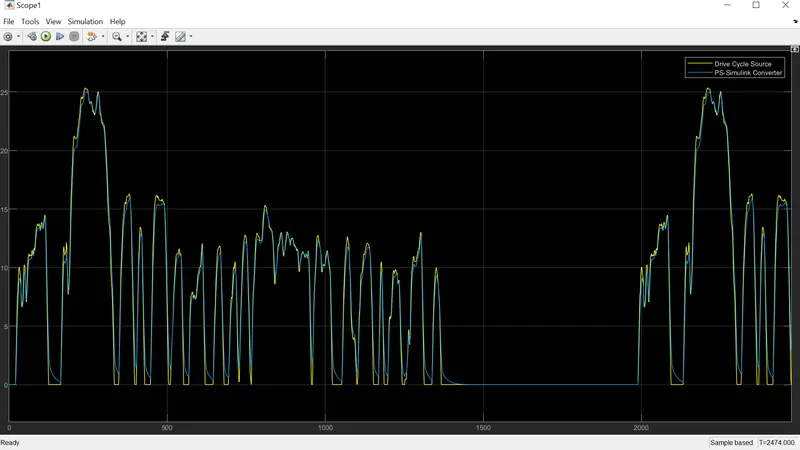
as we observe there are two output graphs in the scope. in that the yellow one is for drive cycle and it contains the data of the drive cycle and the blue one is for the velocity feedback and this contain the data of the velocity feedback with respective to the longitudinal driver feedback. if we see the performance or the graph plotted for the both drive cycle and the feedback velocity looks like in the same region but for not 100% because the drive cycle data is a fixed input data type with out any disturbances but if we see the velocity graph it will be always in lagging position to the drive cycle data because this graph is obtained by running the model and while running the vehicle there may be a sudden breaks and heavy acceleration, road constraints and traffic condition etc.,, many more are considered so due to this reason the velocity graph cannot match with the drive cycle plots.

this is my observation from the above output of the scope from the drive cycle and velocity feedback.

Scope-2 :

below i am attaching the image of the output obtained from the scope which is connected to the SOC terminal of the Battery sub-system

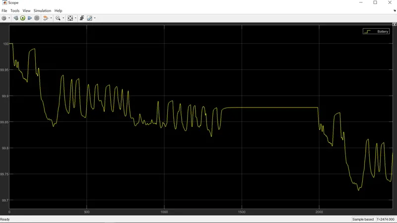
if we observe the above scope the graph of the battery is performing two kinds of operation that is charging and the discharging. iw we observe at the starting the battery is more discharged due to the motor is started and after a particular time it is again charged at some point and then after the battery gets highly discharged due to high acceleration and after like many cycles at approx 1400 to 2000 the graph remains constant because if we observe the drive cycle the vehicle is at rest position so there is not action performed and after that again the charging and discharging modes takes place according to the drive cycle given.

* this is my observation from the above output of the scope pf the SOC terminal of the Battery Sub-system

Scope - 3 :

the below scope is the output graph which i am attaching and it is taken from the current sensor which is in the motor controller sub-system

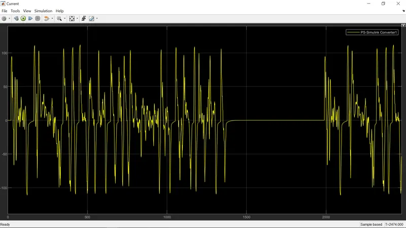
as we observe the current variations in the above graph according to the given drive cycle and the as this current sensor is connected in between the H-bridge and the DC motor it measures the current flowing from the H-bridge to the motor and as we see the number of variations in the output which is fed to the motor from the H-bridge block according to the drive cycle given and due to the acceleration and the deceleration of the vehicle and a continous change in the speed of the motor so, as we observe as the vehicle is in acceleration mode the current flow increases and the flow of current increases as the acceleration is increased and during the deceleration the reverse current is producing, we can see the value as it is in negative state because of the deceleration the battery gets charged

* this is what i observed from the above output scope of the current sensor which is connected in the motor controller sub-system

Scope-4 :

the below scope is the output graph which i am attaching and it is taken from the voltage sensor which is in the motor controller sub-system

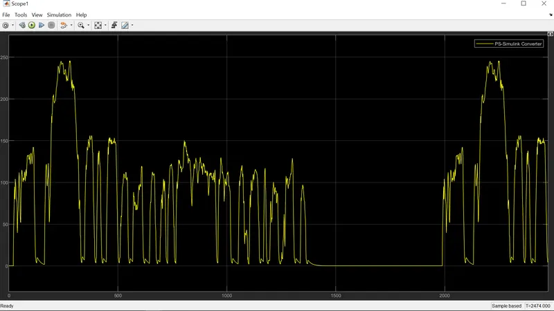
the above output which is obtained from the scope which is connected to the voltage sensor, which is connected in between the motor terminals to know the voltage usage value by the motor during the operation of the model. here if we observe as the vehicle is started it consumes a huge ammount of voltage and the decreased and again with in a little span of time again due to the high acceleration it consumed huge ammount of the voltage and when ever the vehicle is in rest position then no voltage is consumedso, as we observe the change of the voltage consumtion is varied on the change of the velocity of the vehicle

* this is my observation from the above output scope of the voltage sensor in the motor controller sub-system.

Scope- 5 :

the below scope is the output graph which i am attaching and it is taken from the velocity (V) terminal which is in the transmission sub-system

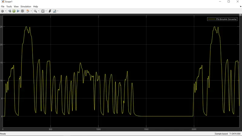
here if we compare the previous scope result of the voltage sensor in the motor controller and the output scope of this velocity terminal scope both looks like similar but there will be minor changes compare to previous one because it shows the voltage consumed according to the velocity of the vehicle but this scope output shows the actual velocity of the vehicle while the model is operated. and this is also related to the drive cycle, if we observe clearly this output is only fed to the Scope-1 which is parallely connected to the drive cycle block and longitudinal block so as we discussed this graph will be in the lagging condition due to the running conditions of the vehicle.

* the above one is my observation from the scope output of the velocity(V) terminal in the transmission sub-system

Conclusion :

1. MATLAB model of electric car using a battery and a DC motor is created.

2. the model is explained and the model is simulated

3. the obtained output scopes are plotted and the output's are explained

4. each and every block is explained and the sub-system's are also elaborated

Note : below i am attaching the SIMULINK (.slx) file of the electric vehicle that is designed. please consider it and refer,

Thank you,

B. V. N. SANDEEP.