Final Project: Design of an Electric Vehicle
Create a MATLAB model of electric car which uses a battery and a DC motor. Choose suitable blocks from Powertrain block set. Prepare a report about your model including following:
Objectives:
1. System level configurations
2. Model parameters
3. Results
4. Conclusion.
Objectives:
- To create a MATLAB model of an electric car by using a battery and DC motor.
- To check out performance parameters: Speed, SOC, Current etc according to the drive cycle.
- To simulate the results.
First will see what is electric vehicle or Electric car and what are the different parts and their function in EV.
Electric vehicle: Electric vehicle(EV)s are increasingly becoming a part of modern life, its tremendous fuel economy, eco friendliness and smooth driving feel have appealed to many consious modern consumers. EVs are quite different from traditional vehicles with internal combution engines(ICE) and from the basic mechanism and operating principle to methods of usage and maintainance. Here wil see the main components of EV and its characteristics. The figure shows the main components of EV
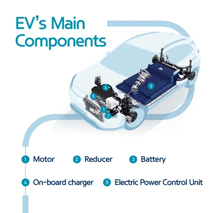
EVs use the electricity saved in the battery to cycle the motor and generate the power necessary for driving, this is the biggest difference to internal combustion vehicles, in which the engine exhausts fossil fuel to generate that power. As in EVs have no need for the engine and transmission. Instead EVs carry several components for electric power; the motor, the battery, the on-board charger and the Electric Power Control Unit(EPCU). All are essential components to achieve the conversion of the batterys electricity into the kinetic force that drives the EV forward.
1.Motor: The motor converts electrical energy into kinetic energy that moves the wheels. The advantage of using the motor instead of an engine is numerous, first the noise and the vibration typically associate with cars are minized. Many passengers riding EV for the first time are surprised by just how quiet and comfortable the ride feels. Morever the EV powertrain is small than the engine, thus providing lots of additional space for efficient vehicle design. The following figure shows the motor used in EV's.
The motor is also in part of an electric generator, it converts the kinetic energy generated while in neutral gear (ex: while the car is going downhill) into electrical energy which charges the battery. The same energy saving applies when the car is reducing its speed, this is called as regenerative braking system.
2.Reducer: The reducer is a kind of mechanism in that it serves to effectively convey the motors power too the wheel. But it carries the name reducer for a reason, the motor has a far higher RPM than that of an ICE, so whereas transmissions change the engine RPM to match the driving circumstance, the reducer must always reduce the RPM to an appropriate level. With the reduced RPM, the EV powertrain can tale advantage of the resulting higher torque. Following image shows the reducer of EV.
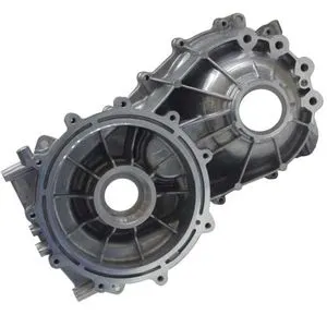
3.Battery: The battery stores electrical energy and is the equivalent of fuel tank in an ICE vehicle. The maximum driving distance of an EV is often detrminded by the battery capacity, the higher the capacity the driving ditance will be higher. Increasing the capacity may seem an obvious choice since high driving distance reduces the annoying need for frequent battery stops at charging stations. But the choice is not so obvious, because the battery size and weight also have large implications on vehicle performance. The larger and heavier battery takes away from cabin/storage space and worsens the enrgy efficiency and fuel economy. The best way to optimize the performance is to maximise the battery's energy density. That is having a small, lightweight battery that stores as much electric energy as possible. The weather affects how much energy your electric car consumes, you have a larger range in summer and smaller range in winter. The following figure shows the battery pack of EV.
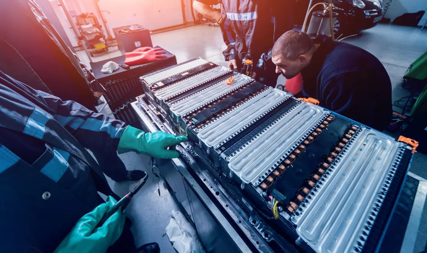
The more recent EVs boast significan upgrades over older models in terms of battery density and driving distance. For example the Kia Soul Booster EV, is equipped with 64kWh Li-ion battery that lasts for the max distance of 386km. The battery life also had signid=ficant improvements, assuming a normal pattern of usage the Soul Booster EVs battery can last through the entire life cycle of the vehicle. To explain in detail, the Li-ion batteries on EV shows the battery life that varies with the charging pattern. If charging pattern is such that the entire battery is exhausted and recharged to full, the battery can be used for 1000charges. If the battery is used to half(50%) and recharged it can be used for 5000charged. If one-fifth of the battert is used(20%) and recharged it used for 8000charges. Means if the Soul Booster EV is driven for 77km per a day (equivalent to the 20% of the max driving distance) and recharged every night, the battery can last for 8000days(22years).
Li-ion battery: Most EVs use Lithium-ion batteries(Li-ions or LIBs). Li-ion batteries have higher energy density, longer life span and higher power density than most other practical batteries. Complicating factors include safety, durability, thermal breakdown and cost. Li-ion batteries should be used within safe temperature and voltage rabges in order to operate safely and efficiently. Increasing the batterys lifespan decreases effective costs. One technique is to operate a subser of the battery cells at a time and switching these subsets.
Battery Management System: The Battery Management System (BMS) manages the battery's many cells so that they can operate as a single entity. The EV battery consistes of as little as tens to thpusand of mini cells, and each cell needed to be in similar condition to the others in order to optimize tha battery's durability and performance. Most often, the BMS is built into the battery's body, though sometimes it is incorporated into the EPCU. The BMS mainly oversees the cell's charge and discharge status, but when it sees a malfuncctioning celll, it automatically adjusts the power status of the cell (ON/OFF) through a relay mechanism(the conditional mechanism for opening/closing the circuits). The following figure indicates the BMS location in the EV car.
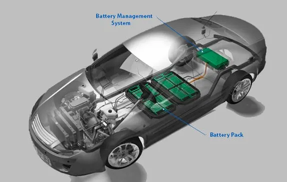
Onboard storage: Power storage methods include; these systems are powered from an external generator plant(nearly always when stationary), and then disconnected before motion occurs, and the electricity is stored in the vehicle untill needed. Chemical energy stored on the vehicle in on-board batteries. Kinetic energy storage in flywheels. Static energy stored ion the vehicle in on-board electric double layer capacitors. Batteries, electric double layer capacitors and flywheel energy storage are forms of rechargeable on-board electricity storage systems. By avoiding an intermediate mechanical step, the energy conversion efficiency can be improved compared to hybrids by avoiding unnecessary energy conversions. Furthermore, the electro-chemical batteries conversions are easy to reverse, allowing electrical energy to be stored in chemical form.
4.Electric Power Control Unit: The Electric Power Control Unit(EPCU) is an efficient integration of nearly all devices that control that flow of the electric power in the vehicle. It consists of the inverter, the low voltage DC-DC converter and the Vehicle Control Unit.
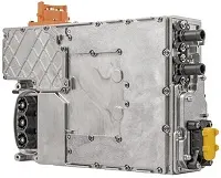
- Inverter: The inverter convers the battery's DC into AC, which is used by an electric motor to control the motor speed. The device is responsible for executing acceleration and deceleration, so it serves a crucial part in maximizing the EV's drivability. The following image shows the inverter of an EV.
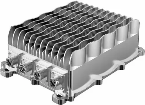
- Low voltage DC-DC converter: It converts the high voltage electricity from the EV's high voltage bettery into low-voltage(12V) and supplies it to the vehicle's various electronic systems. All electronic systems in the EV use electricity in low voltage, so the high voltage in the battery must be converted first to be useful. Follwing figure shows the DC-DC converter used in EVs.
- Vehicle Control Unit: As the control tower of all electric power control systems in the vehicle, the Vehicle Control Unit is the most important component of EPCU. It oversees nearly all the vehicles power control mechanisms, including the motor control, regenerative braking control, A/C load management and power supply for the electronic systems. The following figure sgows the control unit of an EV.
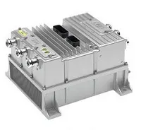
Coming to the controller part, the main function of controller is as a regulator of electrical energy from batteries and inverters that will be distributed to electric motors. Whie the controller itsellf gets the main input from the car pedal. This pedal setting will determine the frequency variation or voltage variation that will enter the motor, and at the same time determine the car's speed. The following figure shows the controller of EV.
Now will see that how an Electric car works: When the car pedal is pressed then, Controller takes and regulates the electrical energy from the batteries and inverters. With the controller set, the inverter then sends a certain amount of electrical energy to the motor according to the depth of pressure on the pedal. Then electric motor converts electrical energy into mechanical energy(rotation). Rotation of the motor rotor rotates the transmission so the wheels turn and then the car moves. (This working principle is for Battery Electric Vehicle(BEV) type).
Charger: Charger is also one of the main component in EV's . It is a battery charging device. Chargers get electricity from outside sorces, such as the utility grid or solar power pants. Ac electricity is converter into DC electricity and then stores in the battery. There are 2 types of electric car chargers. One is On-Board charger, where the charger is located and installed in the car. Second is Off-Board charger, where the charger is not located or not installed in the car.
On-Board Charger: The On-Board Charger(OBC) is used to convert AC from slow chargers or portable chargers used on home outlets into DC. This may make the OBC look similar to the traditional inverter, but they differ in function-the OBC is for charging and the inverter is for acceleration/deceleration. Incidentaly the OBC is not needed in ast charging, since fast chargers already supply the electricity in DC. The following figure shows the 6.6KW liquid cooled on-board charger used in EV's.
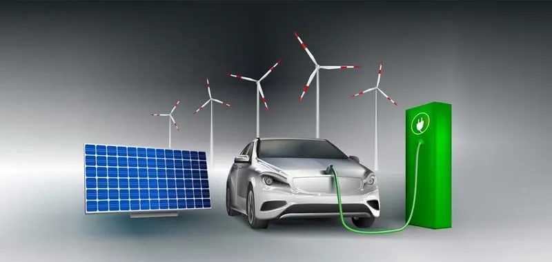
Electric cars function by plugging into a charge point and taking electricity from the grid. They store the electricity in rechargeable batteries that power an electric motor, which turns the wheels. Electric cars accelerate faster than vehicles with traditional fuel engines, so they feel lighter to drive. Which is also called ass Off-Board charging. The charging port allows the vehicle to connect to an extenal power suppy in order to charge the traction battery pack. The following figure shows the different resources for charging of an EV.
To facilitate higher power charging, which requires much larger AC-DC coonverters, the converter is built into the charging stations instead of the vehicle and the station supplies already converted DC power directly to the vehicle, bypassing the vehicle's onboard converter. These are known as DC charging stations. Most fully Electric car models can accept both AC and DC power. Chargig stations provide connectors that conform to a variety of standards. Dc charging stations are commonly equipped with multiple connectors to be able to supply a wide variety oof vehicles. Folowing figure shows the chrging station for EV's.
There are also 3 main EV charging speeds. They are,
- Slow: Typically rated up to 3kW, Often used to charge overnight or at the workplace. Charging time is 8-10hours.
- Fast: Typically rated at either 7kW or 22kW. Tend to be installed in car parks, supermarkets, leisure centres and houses with off-street parking. Charging time is 3-4hours.
- Rapid: Typically rated frpom 43kW. ONly compatible with EV's that have rapid charging capability. CHarging time is 30-60minutes.
Which is indicated through the following figure.
Energy Efficiency: EV tank-to-wheels efficiency is about a factor of 3 times higher than ICE vehicles. Energy is not consumed while the vehicle is stationary, unlike ICE which consume fuel while idling. However, looking at the well-to-wheel efficiency of EVs, their total emissions, while still lower, are closer to an efficient gasoline or disel in mosr countries where electricity generation relies on fossil fuels. A particular EV would instantlyy become twice as efficient if electricity production were switched from fossil fuels to renewable energy, such as wind power, tidal power, solar power and nuclear power.
How far you can travel on a full charge depends on the vehicle. Each model has a different range, battery size and efficiency. The perfect car for you will be the one you can use for your normal journeys without having to stop and charge up halfway through.
Block diagram: The block diagram shows the schematic form of general arrangement of the principle parts of an electric car. The following figure shows the block diagram of our MATLAB model of an electric car. Where it is showing the 6 main parts of an arrangement.
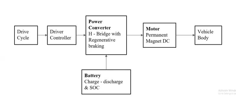
Where the Drive cycle is used to input the data into the driver controller. The driver controller controlls the acceleration and deceleration of the vechile. Power converter which is a H-Bridge with regenerative braking, here the H-Bridge is used to drive the Dc motor. As per our model we are using a battery and dc motor. So where the battery block indicates the charge and discharging condition and the %of SOC (state of charge) variations with respect to the drive cycle. The motor block and battery block is connected to the power converter block which indicates that, power converter plays a vital role in the controling and converting the electrical energy. Motor block indicates the motor positioining and type of motor we are using, here we are using the permanent magnet DC motor. And finaly the vehicle body block indicates the mechanical structure of an electric car like wheels and their connections.
MATLAB modelling:
Coming to the MATLAB model, I have created a MATLAB model of an electric car by using the battery and DC motor by choosing the suitable blocks from the powertrain blockset and i have modeled its parameters. The following figure shows the Simulink model of an electrical car.
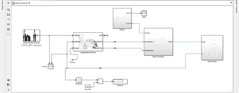
According to the block diagram i have arranged all the blocks in a clear and detailed manner. Where the motor controller, vehicle body and battery has subsystems which will be explained clearly in the following description along with the blocks used to model the system.
DESCRIPTION OF MODELLING & CONNECTIONS: In the description of modelling will explain the each block one by one with the parameters we are used and connections we have made. First will see about the Drive cycle source block.
Drive Cycle Source: The Drive cycle source block generates a standard or user specified longitudinal drive cycle. Here in our model we are using the standard drive cycle. It's output is the specified vehicle longitudinal speed, which is used to predict the engine torque and fuel consumption that a vehicle requires to achieve desired speed and acceleration for a given gear shift reference. It produce realistic velocity and shift references for closed loop acceleration and braking commands for vehicle control. It identifies the faults within the tolerences specified by standardized tests. Drive cycle source optimize the vehicle control,system performace and system roboustness over multiple drive cycles. The Drive cycle source block looks like in in the following image.
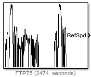
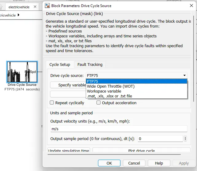
Drive cycles are predefined source. By default the block includes,
- FTP75 drive cycle, which is used in our model. Generally it is upto 2474seconds.
- Wide Open Throttle(WOT) parameters including intial and nominal reference speed,seceleration start time and final reference speeed.
- Workspace variables that desines our own drive cycles, we have to create it by our self by selecting the option we can load our data into it.
- We can also enter the data through .mat, .xlx, .xlsx, or .txt files.
Where the refspd port is connected to the longitudinal block. The following figure shows the block parameters of the Drive cycle source block.
Longitudinal Driver: This block implements a longitudinal speed tracking controller. Based on reference and feedback velocities, the block generates normalized acceleration and braking command that can vary from 0 to 1. The following image shows the longitudinal driver block.
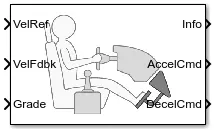
Where the input ports are: velref which is connected to the drive cycle source block for the reference velocity, VelFdbk port is a feedback port connected from the vechilce body gear. Grade is grounded. Info is connected to terminator block. AccelCmd is connected to the respective acceleration sorce and Decelcmd is connected to its respective deceleration sorce. In the Longitudinal block we have selected the control type as PI. The following figure shows the block parameters of the block.
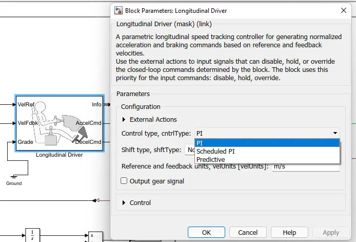
PI means Proportional Integral control with tracking windup and feed-forward gains. For the sheduled PI configuration, the block used feed forward gains that are a function of vehicle velocity. To calculate the speed control output, the block uses the following equation,
y = (Kff/Vnom)×Vref + (Kp×Eref)/Vnom + ∫[(Ki×Eref)/Vnom + (Kaw×Eout)]×dt + Kgθ
where,
Kff = Velocity feed forward gain
Vnom = Nominal vehicle speed
Vref = Reference velocity signal
Kp = Proportional gain
Eref = Velocity error
Ki = Integral gain
Kaw = Anti-windup gain
Eout = Difference between saturated and nominal control outputs
Kg = Grade angle feed-forward gain
θ = Grade angle.
Motor Controller Subsystem: Motor controller is a subsystem, which consists of following desined model shown in the figure. This subsystem controlls the motor actions it is connected in between the vehicle boody and longitudinal block and also had a connection with the battery. It plays a major role. Which is used to control the motor speed and to charge and discharge the motor according to the motoring and braking conditions.
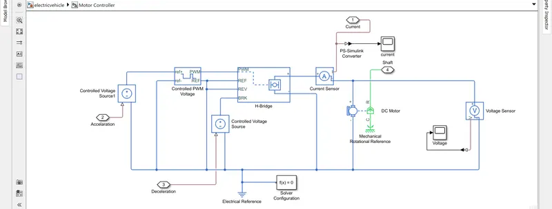
This subsystem consists of many blocks will see one by one. The block used are,
Controlled voltage source,
Controlled PWM voltage,
H-Bridge,
Current sensor,
Voltage sensor,
Dc motor,
Solver configuration,
PS-Simulink converter,
Electrical reference,
Mechanical reference,
Scope,
Connection ports.
Now will discuss each block and its parameters.
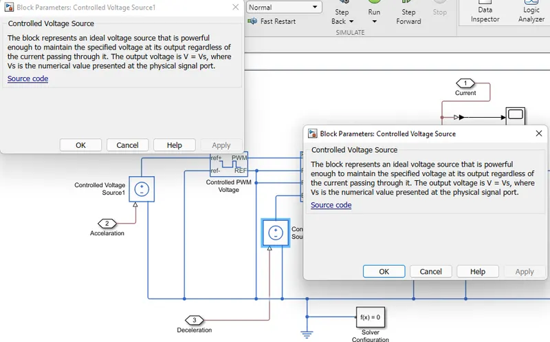
Controlled voltage source: The controlled voltage source block represents an ideal voltage source that is powerful enough to maintain the specified voltage at its output regardless of the current flowing through the source. The block has one physical signal input port and two electrical conserving ports associated with its electrical terminals. The block is shown in the following image.

Here we are considering the 2 controlled voltage source blocks.
In case of controlled voltage source1 block, the positive terminal is connected to the positive reference terminal of the Controlled PWM voltage block and the negative terminal is connected to the common ground. The physical port is connected to the connection port2 which indicates the acceleration. This port is connected to the Accelcmd port of longitudinal driver.
In case of controlled voltage source block, the positive terminal is connected to the Break port of H-Bridge block and the negative terminal is connected to the common ground. The physical port is connected to the connection port3 which indicates the deceleration. This port is connected to the Decelcmd port of longitudinal driver.
The following figure shows the both blocks indication.
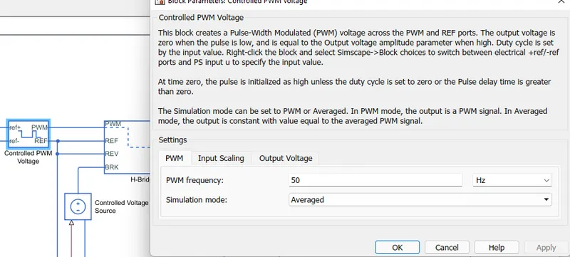
Controlled PWM voltage: The controlled PWM voltage block represents a pulse width modulation(PWM) voltage source. The block has two modeling variants fo the simulation that is PWM and Averaged. In our model we are selecting the simulating mode as averaged. Simulating the motor with an averaged signal estimates the motor behaviour in the presence of a PWM signal. The bock calculates the duty cycle based on the reference voltage across its positive ref and negative reference ports. This modeling is the default. The following image shows the controlled PWM voltage block.

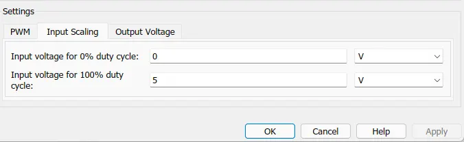
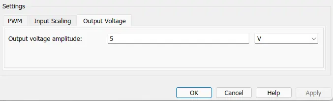
Where +ref port is connected to the controlled voltage source, PWM port is connected to the H-Bridge PWM port. -ve ref and REF ports are connected to the common ground(REF port is also connected to the REF port of H-Bridge). The following images shows the parameters we have modeled. PWM frequency as 50Hz, simulation mode as Averaged. Input voltage and output voltage is set as 5V.
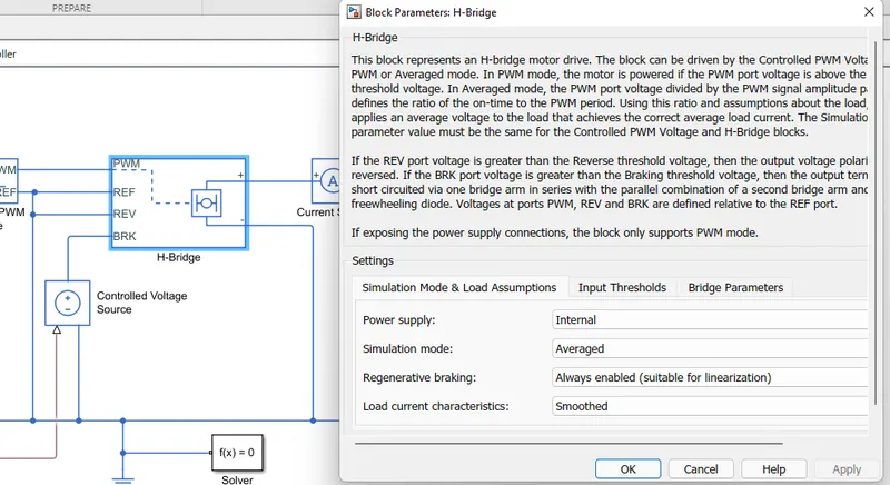
H-Bridge: The H-Bridge block represents an H-Bridge motor driver. In this block also we have selected the simulation mode as averaged. When H-bridge block with a controlled PWM voltage block is considered it is efficient to slect the simulation mode as averaged in both the blocks. This applies the average of the demanded PWM voltage to the motor. The accuracy of the averaged mode simulation results relies on the validity of our assumption about the load current. Braking mode is involved when the voltage presented in the BRK port is larger than the Braking threshhold voltage. Regardless of whether in PWM or averaged mode. The following image shows the H-Bridge block.
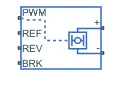
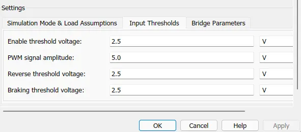
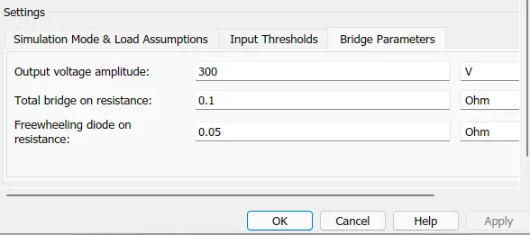
Where PWM and REF ports are connected to the respective ports of controlled PWM voltage block. REV port is connected with the REF port to the common ground. BRK port is connected to the positive terminal of the controlled voltage source to indicate the deceleration during the braking period. The ouput +ve and _ve ports are connected to the DC motor along with the current sensor. The following figures shows the modeled block parameters of H-Bridge block.
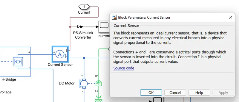
Current sensor: The current sensr block represents an ideal current sensor, i.e, a device that converts current measured in any electrical branch into a physical signal proportional to the current. The connections +ve and -ve are electrical ports through which the sensor is inserted in between the H-bridge and DC motor. Connection I is a physical signal output port for the measurement of result current. Which is connected to the scope block by using the PS-simulink converter. The scope block shows current variations accordig to the drive cycle data.

The following figure shows the connections of current sensor. Where a connection port 1 is taken to connect the connection to other subsystem block.
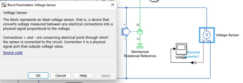
Voltage sensor: The voltage sensor block represents an ideal voltage sensor, i.e, a device that converts voltage measured across the motor into a physical signal proportional to the voltage. The +ve and -ve connections are technical conserving ports through which the sensor is connected to the the circuit. The port V is a physical signal port that outputs the measurement result of voltage across motor. Which is connected to the scope through the PS-simulink converter. The voltage sensor block is shown below.
The following figure shows the connection of voltage sensor across DC motor and connection to the scope block.
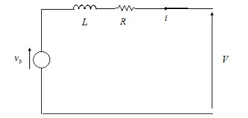
Dc motor: The DC motor block represents the elctrical and torque characteristics of a DC motor using the following equivalent circuit model. Where the circuit has armature inductance and resistance elements. We can model these parameters according to our requirement or according to our selected model.
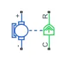
The following image shows the DC motor block. Where +ve and -ve connections ar electrical which are connected to the H-Bridge and C, R are the mechanical ports which are connected to the respective mechanical gear. We have taken a connection port across it to connect it further with the mechanical system. Taking the connection port4 as Shaft.
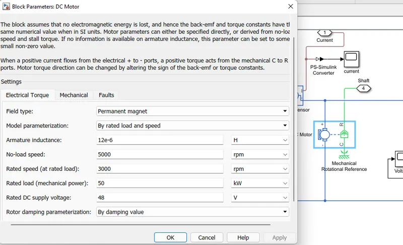
Here we are selecting the model parameterization as By rated load and speed. Which provides power and speed parameters that the block converts to an equivalent model of the motor. The following figure shows the block parameters and its connections. Selected faults as NO.
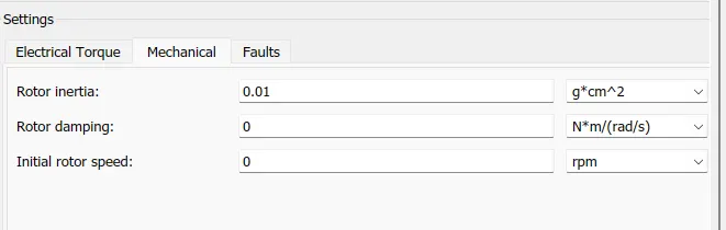
Solver configuration: The solver configuration block is shown in the following image. Each physical network represented by a connected simscape block diagram requires solver settings information for simulation. It specifies the solver parameters that our model needs before we can begin simulation. Each topologically distinct simscape block diagram requires exactly one solver configuration black to be connected to it.

The block has one conserving port. We can add this block anywhere on a physical network circuit by creating a branching point and connecting it to the only port of the solver configuration block. In our model i have connected the solver configuration block at the common ground terminal.
PS-Simulink converter: The PS-simulink block converts a physical signal into a simulink output signal. We used this block to connect outputs of a physical network blocks like current and voltage sensor blocks to simulink scopes. The following images shows the PS-simulink converter.

The block has a physical signal input port at left side and simulink output port at right side(from the above figure).
Electrical reference: The electrical reference block represnts an electrical ground. This block has only one electrical conserving port. Electrical conserving ports of all the block that are directly connected to ground must be connected to an electrical reference block. Following images shows the image of electrical reference block.

Mechanical rotational reference: The mechanical rotational reference block represents a reference point for mechaical rotational ports. Rotational parts are rigidly clamped to the ground must be connected to a mechanical rotational reference block. In our model the mechanical part of DC motor is connected to this block. This block also has only one mechanical rotational port which is shown in the below figure.

Scope: The following image shows the scope block. Through the scope block we can observe the resultant plots. We can add the additional ports to view the another plots in one scope block. We can select the legend option in the plot to view the name of the plot. Ans we can set the layout to view the different plots.

Connection ports: The connection port block, placed inside a subsystem created an open round physical modeling connector port  on the boundary of the subsystem. When it is connected to a connection line, the port becomes solid . You can connect individual blocks and subsystems to one another with connection line instead of normal simulink signal lines. You can add additional connector ports by adding connection port to your suubsystem. The following images shows the connection port. BY adding additional connection ports the number increases. Where the acceleration and deceleration ports are connected to the respective ports at the longitudinal driver block.

Battery Subsystem: The batteru subsystem includes a battery to supply the electrical energy to the motor to run efficiently. And a circuit to calculate the SOC(State of charge) variations. Now will see all the connection made unde the battery subsystem. The following figure shows the connections under the battery subsystem.
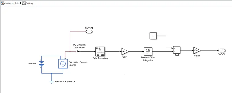
Where the ports used are,
Battery,
Controlled current source,
Electrical reference,
To calculate the SOC the following blocks are used,
Rate transition,
Gain,
Discrete time integrator,
Add block,
Connection ports,
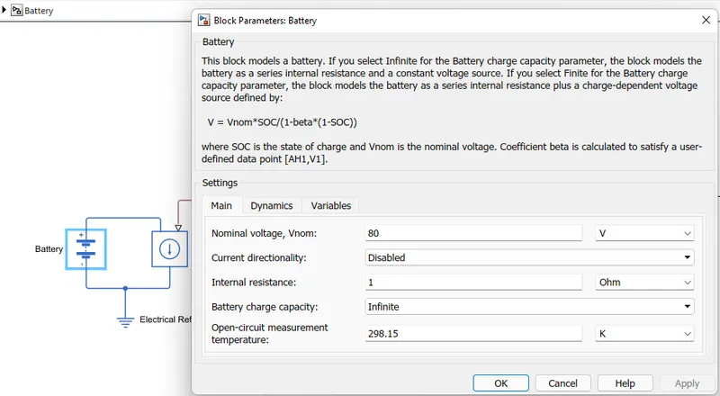
Battery: The battery block represets a simple battery model, which is shown in the following figure. Where the positive and negative terminals of the battery is connected to the controlled current source and to the ground which is connected to electrical refernce block respectievely. Battery plays a major role in the Electric cars as they are run by the battery supply. We can check the battery charging and discharging conditions according to he motoring and braking actions. In the braking mode the battery gets charged.

The following figure shows the block parameters and connections of the battery. Where the dynamica and variables are kept as usual.
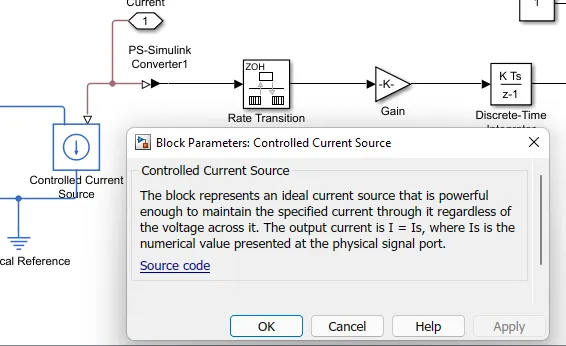
Controlled current source: The controlled current source block represents an ideal current sorce that is powerful enough to maintain the specified current through it regardless of the voltage across the source. Where the controlled current sorce block is connected acrss the battery. The following figure shows the controlled current source block.

This block has one physical signal inputport and 2 electrical ports associated with its electrical terminals. The following figure shows the connection of the block. Where the physical port is connected to rate transition block by using PS-simulink converter. The connection port1 taken across it is connected to the cmottor controller current connection port1
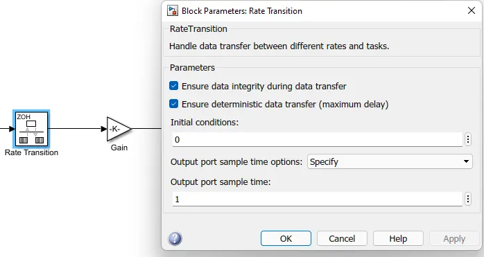
Rate transition: The rate transition block transfers the data from the output of a block operating at one rate to the input of a block operating at a different rate. By using the block parameters we can trade data integrity and deterministic transfer for faster response or lower memory requirements. In our model it transfers data from the battery current to calculate the SOC of the battery. The following image shows the rate transition block.

It has one input and one output port. And the following figure shows its connection and parameters.
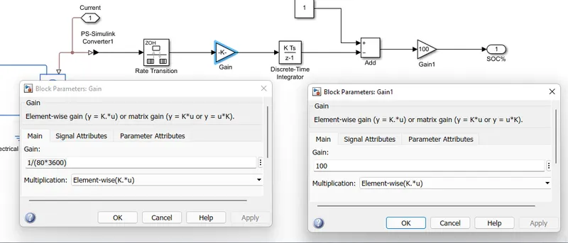
Gain: The gain block multiplies tha input by a constant value. The following image shows the gain block. It has only one input and output port.

In our model we are using 2 gain blocks, the connections and parameters of those 2 blocks are shown in the following figure.
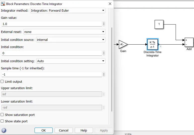
Discrete time integrator: The discrete time integrator block used in place of an integrator block to create a purely discrete model. With this block, we can define intial conditions, input gain value, upper and lower limits on the integral. The following figure shows the discrete time integrator block.

This block also had only one input and one output port. The following figure shows the connection and parameters of the block.
Add Block: The addition block is used to add the input values and give the result through its output. Here we are taking 2 inputs one is from the discrete time integrator and another from the constant valu1 from the constant block. And giving its output to the gain block which further connects to the connection port.
Electrical reference and Connection ports are already discussed above. Connectionnport1 is connected to the current of connection port1 in the motor controller subsystem. And connection port %SOC is connected to the scope block to observe the variation in state of charge which is the ratio of current charge to rated battery capacity.
Transmission Subsystem: The vehicle body subsystem consists of four wheels which are connected to the vehicle body of the electric car. And this subsystem shows the mechanical action between the wheels and gear. The following figure shows the simulink model of vehicle body subsystem.
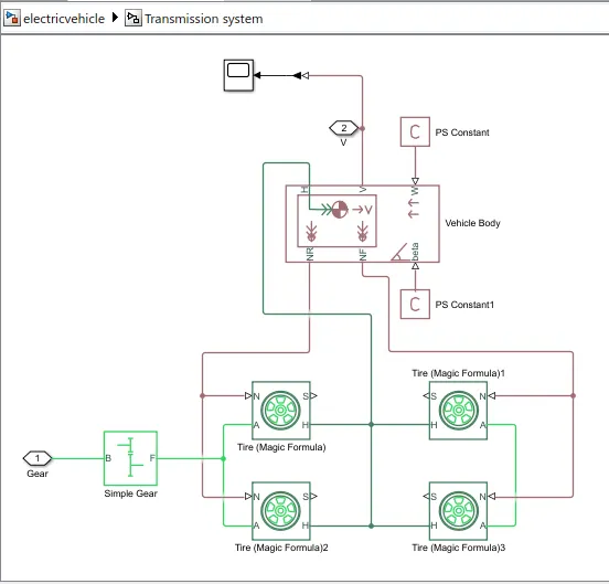
The blocks used in this subsytem are,
Tire(magic formula),
Vehicle body,
Simple gear,
PS constant,
PS to simulink converter,
Scope and connection ports.
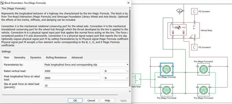
Tire(magic formula): The Tire(Magic formula) block models a tire with longitudinal behaviour. The block can model tire dynamics under constant or variable pavement conditions. The longitudinal direction of the tire is same as its direction of motion as it rolls on pavement. This blocck models the tire as a rigid wheel-tire combination in contact with the road and subject to slip. When torque is applies to the wheel axle, the tire pushes on the ground and transfers the resulting reaction as a force back on the wheel. This action pushes the wheel forward or backward. The following image shows the Tire(Magic formula) block.

Where the port indicates that,
N - It is a physical signal input port associated with the normal force acting on the tire.
A - It is a mechanical rotational port associated with the axle that the tire sits on.
S - It is a physical signal output port associated with the relative slip between the tire and road.
H - It is a mechanical translational port associated with the wheel hub that transmits the thrust generated by the tire to the remainder of the vehicle.
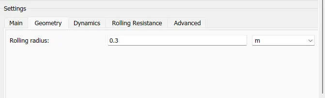
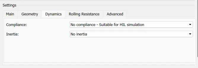
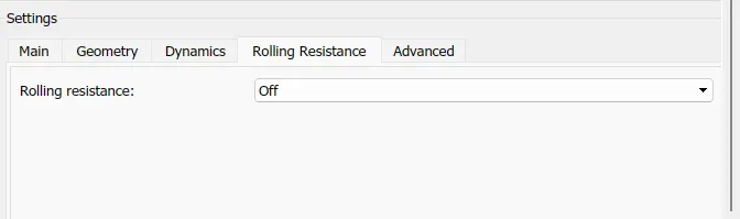
In our modelling of an electric car we require four tires, so we have taken the 4 blocks which are configured equally. The parameters which are configured is shown in the following figures. Coming to the connections of tires,The N port of the left side two tires are connected together to the NR port of the vehicle body and N port of the right side two tires are connected together to the NF port of the vehicle body, which indicates the rear and fron wheels respectievely. All the H ports of the 4 tires are connected to the H port of the vehicle body. The A ports of left side tires are connected in the same manner the right side tires A ports are also connected. Simple gear block is connected to the common A port of the left side tires as shown in the following image.
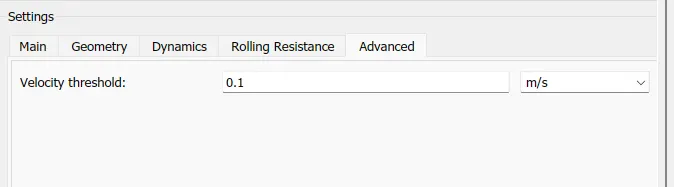
Vehicle Body: The vehicle body block represents a two-axle vehicle body in longitudinal motion. The vehicle can have the same or different number of wheels or tires on each axle. In our model we are taking two tires on each axle. The vehicle tires or wheels are assumed identical in size, as we discussed above. The block accounts for body mass, aerodynamic drag, road incline and weight distribution between axles due to aceleration and rooad profile. The vehicle body is used as a control mechanism. The following image shows the vehicle body block.
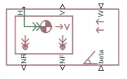
The ports of vehicle body are,
NR - It is a physical signal output port for normal force on the rear axle. Wheel forces are considered positive if acting downwards.
NF - It is a physical signal output port for normal force on the front axle. Wheel forces are considered positive if acting downwards.
Beta - It is a physical input port for road incline angle.
H - It is a conserving port associated with the horizontal motion of the vehicle body. Tire traction motion is connected to this port.
V - It is a physical signal output for vehicle longitudinal velocity.
W - It is a physical signal input port for headwind speed.
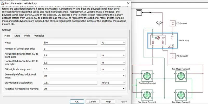
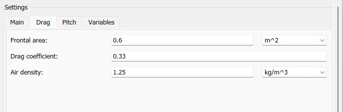
Where NR is connected to the left side tire N ports and NF is connected to the right side tires N ports. H is connected common to all the tires H ports. Beta and W is connected to PS constant blocks. V is connected to the scope block through PS-simulink converter. The scope block displays the vehicle longitudinal velocity. Connection port2 is taken across the V port which is connected to longitudinal driver block as the feedback velocity.The connections and the parameters used in our model is shown in the following images. Where pitch and variables are kept as usual.
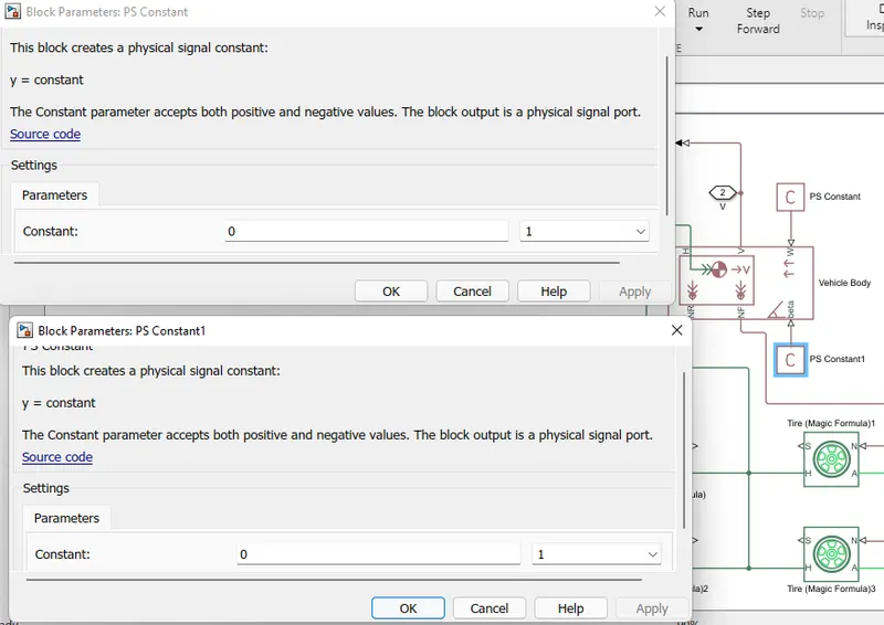
PS Constant: The PS Constant block generates a physical signal of a constant value. This lock has only one output port which is a physical signal. The following figure shows the images of PS Constant block.

We specified the value and unit of the signal as the constant parameter. In our model we have used two PS Constant blocks. WHich are connected across the W and Beta ports of the vehicle. The connection and the constant parameters we specified is shown in the following figures.
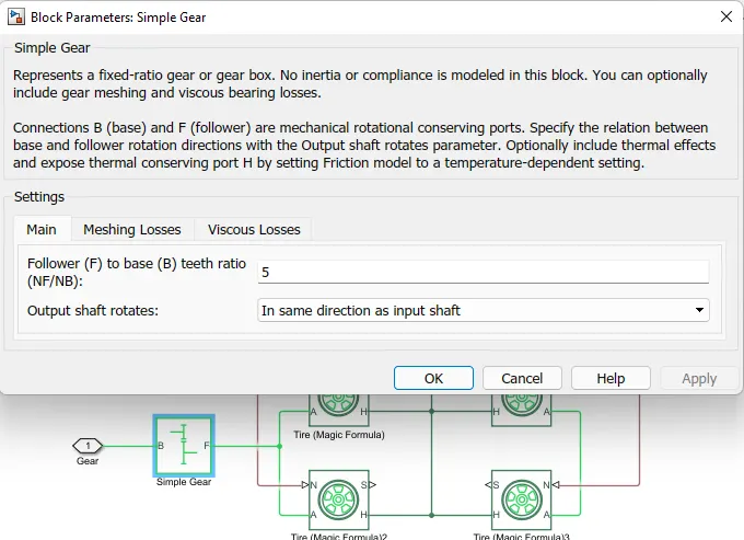
Simple gear: The simple gear block represents a gearbox that constrains the connected driveline axes of the base gear B, and the follower gear f, to corotate with a fixed ratio that we specified. We can choose the follower axis rotation, which is either in the same or opposite direction as the base axis. If they rotate in same direction, the angular velocity of the follower and angular velocity of the base have the same sign. If they rotate in opposite directions, the angular velocities have opposite signs. In our model we are considering the same direction as base axis. The following figure shows the image of simple gear block.

where the ports represents,
B - It is a rotational mechanical conserving port associated with the base, or input shaft.
F - Its is also a rotational mechanical port associated with the follower, or output shaft.
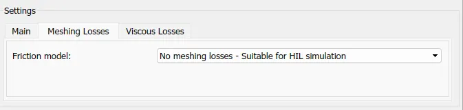
The Port F is connected to the common connection of rear tires A port. And the port B is connected to a connection port as gear which is connected at the shaft connection port in the motor controller subsystem. Which means this gear port is connected to the DC motor R port. The connections and the parameters we have modeled are showsn in the following figure. Where the viscous losses are kept as usual.
PS-Simulink converter, Scope and Connection ports are already discussed above and their connections also described at the respective block.
Connections and the parameter configurations are described. Now will see the down part of the main simulink model which is taken to calculate the total distance covered by the vehicle. The following figure shows the connections we have made to calcuate the distance.
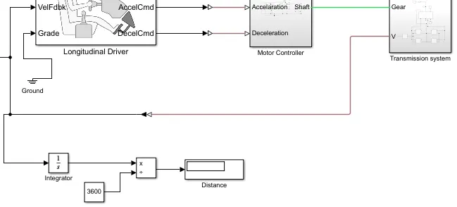
In the above figure we have taken a integrator block at the velocity feedback port. Because when velocity is integrated with respect to time will get the total distance covered from intial position to final position. Here we are taking a constant block to divide with 3600 which gives the distance per second. Here the integrator block and constant blocks are multiplied and divide accordingly and finally will get the distance in m. Which is displayed in the display block which is named as distance. If we divide with the constant value 1000 wil get the distance in Kilometers.
SIMULATION: Now coming to the simulation part, we have a drive cycle for 2474seconds, we can change simulation time according to that. In our model iam considering the complete simulation time to observe the complete performance according to the source. So, now iam running the model by selecting the stop time as 2474sec by clicking on the run button at the top of the window. So we can see the following observation which is shown in the figure.
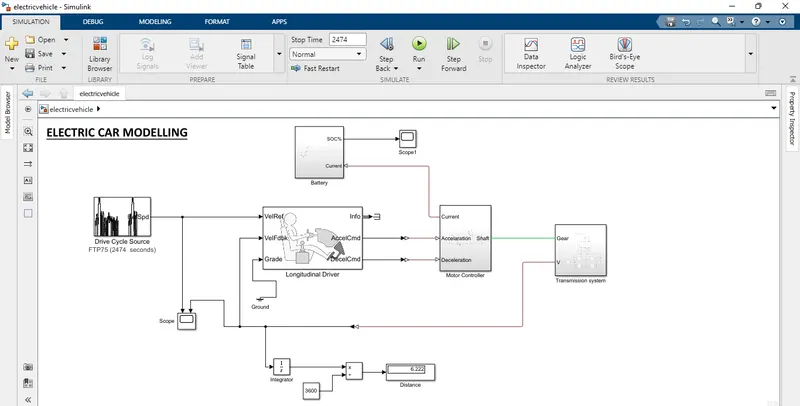
So we can observe the stop time i have taken at the top of window, and we can see the the distance covered by the electric car we have modeled in the display block. It is 6.222meters per second and if we want to check the result in kilometers, we can simply change the constant value to 1000 and then run again, where will get the total distance covered by the car in kilometers. By converting meters to kilometers we can say that it is nearly 22.4kilometer per hour. We even can observe the distance covered according to the time variation during the running process. Like after it is compiled we ca observe the changes in distance at display block with respect to time. I have taken a snip in the middle of running process to show it clearly we can observe the following figure.
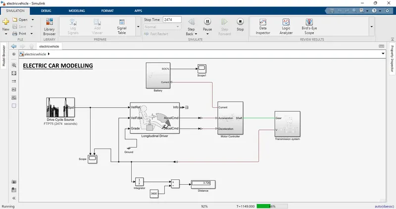
The above figure shows the distance of the vehicle during the running process which is at 46% of the stop time that is at 1149seconds, it can be observed as 3.726meters. So during the simulation process we can observe the distance travelled by the car with respect to time. The distance is measured from the velocity feedback supply. Whatever the speed the vehicle is running which is given as a feedback to the longitudinal driver block. From there we can measure the distance by integrating the speed. Now will check the simulation results of different parameters at the respective scope blocks.
RESULT: The resultant plots are shown in the following figures.
1. The following plot has been observed from the scope which is connected across the Drive cycle source and feedback velocity which is coming from the transmission subsystem to the longitudinal driver block.
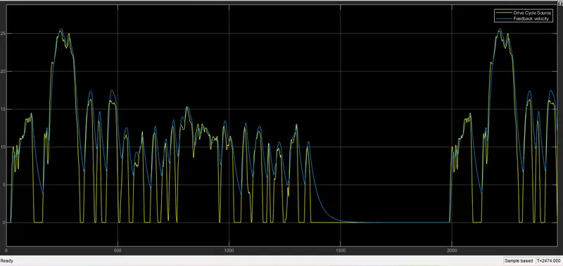
From the above figure we can observe the two different plots one is the input data source which is given by the drive cycle source and another one is the feedback velocity. Which are indicated through two colours, mentioned as the legend at the top right corner of the plot. Yellow plot represents the drive cycle data and Blue plot represents the actual velocity whichi is fedback to the longitudinal driver block. If we observe them we can say they are looking similar but not exactly. Because when we driving the car there will be speed variations according to the time, sudden stops, and some other factors also effects like type of road and rollling resistance etc., so there will be same movements like high speed, low speed but due to the factor effected in the real time there will a variation from the original drive cycle.
2. The following plot has been observed from the scope block which is connected at the battery subsystem.
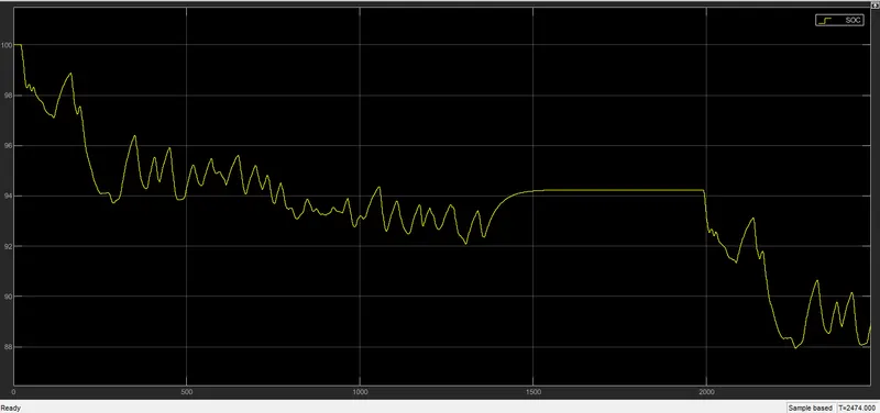
The above plot represents the variations in state of charge(SOC), that is charging and discharging conditions of the battery. If we observe and compare the first plot with this SOC plot, it shows that when the car is accelerating to high value the battery is discharging and when it is in decelerating condition the battery gets charged. In deep we can clearly observe this: approxly at 250sec there is a sudden increase in acceleration which is from the first plot, at the same time if we observe in the second plot i.e. in SOC plot we can see that there is discharging condition. Again if we observe from 1500-2000sec in the first plot the car is decelerating and it is almost zero which means either the car is in neural gear or it is in downhill road, Where in the SOC plot in that time duration the battery gets charged constantly.
3. The following plot can be observed from the scope which is connected in the motor controller subsystem at the current sensor block.
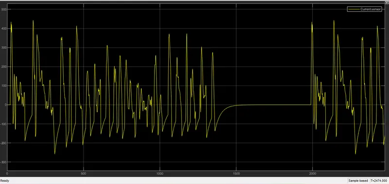
The above plot shows the current variations of the motor according to the drive cycle. The current sensor which is connected in between the H-Bridge and DC motor senses the current changes and they are ploted through the scope block. So this current variations are observed from the changes in DC motor conditions. If we analyse the data by comparing with the first plot, we can see that the current is incresing according to acceleration and decreasing according to the deceleration. And if the vehicle is maintaining a constant acceleration or deceleration then the current is also minting it range according to it. If we observe the peak value, that is if the vechile is at the velocity of 25m/s where the current is at almost 450A, and if we observe it at neutral condition that is at 0 velocity the current value is also settled at constant zero value. And during decelerating of the car the current value is also going to decrease in negative values.
4. The following plot has been observed from the scope which is connected in motor controller subsystem across the voltage sensor block.
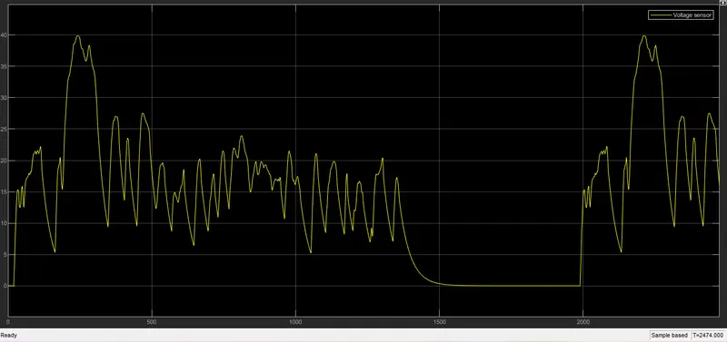
The above plot shows the voltage variations of the motor according to the car accelerating and decelerating conditions. This voltage sensor block is connected across the motor to observe this variations. If we compare it with the resultant plot of velocity feedback, it can be say that there is changes in voltage with respective to the velocity changes. If the vehicle is accelerating condition the voltage is also increasing and when the vehicle is decelerating condition, the value of voltage is also decresing and when the car is maintaining its velocity at certain pont with respect to time, the voltage is also maintaining its constant value with respective to the velocity feedback.
5. The following plot has been observed from the scope which is connected in the transmission subsystem across the vehicle body: longitudinal velocity port.
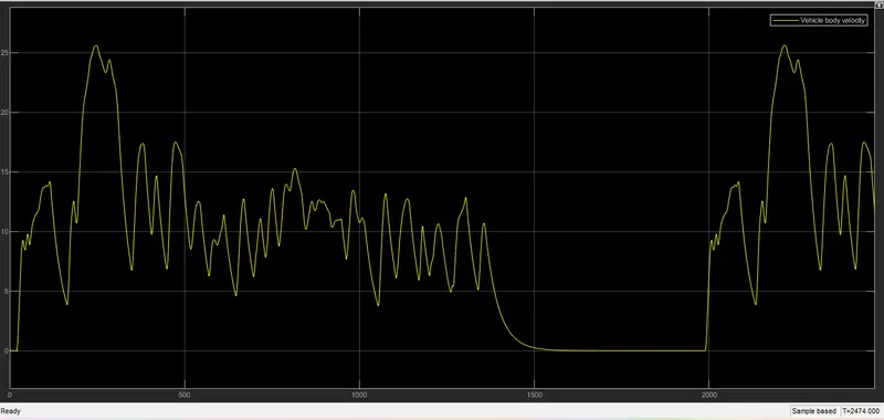
If we observe the above two plots they are almost similar. Because as we discussed in the fourth plot, the velocity variations and voltage variations are proportional to each other. As this plot is observed from the block which is conected to the vehicle body, it gives the actual velocity changes happened in the vehicle. In the first plot the velocity observed is this feedback velocity which given to the longitudinal block. So it is clear that if the acceleration increases its velocity increases and if it the acceleration of the vehicle is decreasing then the value of velocity is also decreases.
CONCLUSION: MATAB model of an electic car is created by using the DC motor and Battery. It is simulated and the results also has been plotted. The performance of different parameters are discussed step by step. The modelling is also explained clearly with the blocks used. The connection between the different blocks and the function of each block is also described.