The electric vehicle overall block diagram can be as shown in the figure.

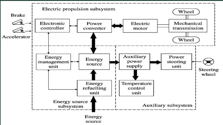
An electric vehicle consists of three subsystems: Electric propulsion subsystem, energy source subsystem, and auxiliary subsystem.

An electric subsystem receives the command from the driver as per the input, which goes to the electronic converter that converts the driver's input to logic signals that are given to the power converter to dive the motor connected to it. The Motor shaft is connected to the transmission and differential.

The energy source subsystem has an electronic management unit that controls the energy transmission between the battery source and the power converter. An auxiliary supply goes to the auxiliary subsystem to power up other essentials of the vehicle.

The MATLAB model of an electric car is given below

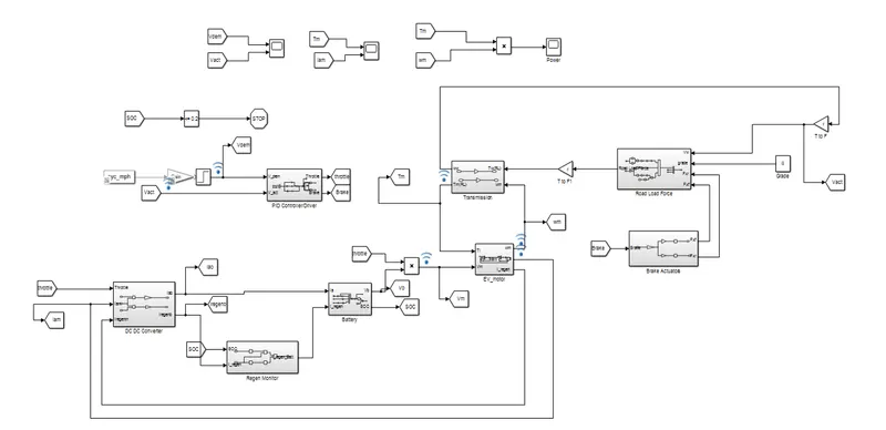
Electric Vehicle consists of various parts which should work in correlation to achieve optimized performance. Here, various parts are divided into different subsystems and are modeled based on the mathematical relation between their input and output. All of these subsystem domains are integrated to form the overall electric vehicle design.

A. Electric Motor Subsystem

An electric motor is the most important component of an EV as it drives the whole vehicle depending on the power received by the motor. This paper uses a Permanent magnet DC motor to achieve its goal.

The motor can be divided into electrical and mechanical equations. The equivalent circuit of the motor is shown in Fig1.

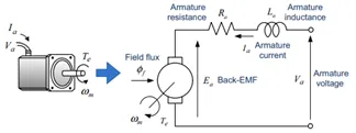
Using Kirchhoff’s Voltage Law,

V=R×i+L di/dt+V_e                                           

Where, V is Voltage applied, R is armature resistance, i is the current flowing, L is the inductance, Ve is the back emf generated.

According to Lenz's law, the emf induced in the circuit is due to the change in magnetic field is directed to oppose the change in flux given by

V_e= K_e×dθ/dt 

eq(1.2)

Where Ke is the back emf constant.

Rearranging

di/dt=1/L (V-R×i-K_e×ω)

eq (1.3)

Where ω is the rotor speed

The effective torque (Te) given by the mechanical relation,

T_e=J dω/dt+B×ω+T_L        

eq (1.4)

According to Lorentz law, a current-carrying conductor placed in the magnetic field experiences a torque (Te) given by

    T_e=K_t×i          

eq (1.5)

Where Kt is the motor torque constant, is the load torque and is the coeffiecient of friction .

Rearranging

J dω/dt=K_t×i-B×ω-T_L                         

eq(1.6)

The effective velocity of the motor is achieved by,

dω/dt=1/J (K_t×i-B×ω-T_L )                      

eq (1.7)

The inductance (L) resists the change in current. The inductance in the motor consumes voltage and reduces the peak motor speed while producing torque and reducing the measured motor current. Internal Resistance( R) is due to the armature windings. Lower R causes lesser energy loss and is mostly preferred. The modeling is done by taking applied voltage and load torque as input and angular speed as output.

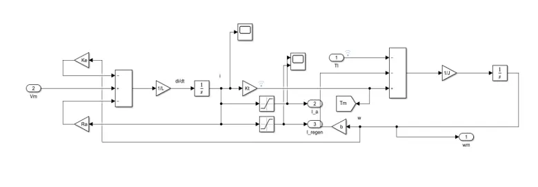
As shown in Fig two saturation blocks are connected at the current terminal: the positive saturation limits are given to armature current and the negative saturation limits are given to the regeneration current.

B. Battery Subsystem

The EV industry is continuously focusing on the development of Battery Technology. The model helps in understanding the key parameters of the battery using the basic equations.

∫〖I_a dt=  Q_a   and ∫〖I_regen dt〗=Q_regen  〗

(2.1)

The total available charge is given by

Q_available=Q_initial-Q_a+Q_regen  

(2.2)

is the maximum charge available at the time of start.

The SOC of the battery is given by

SOC=Q_available/Q_maximum                                                   

(2.3)

A saturation block is added to ensure the SOC remains positive. The Battery model subsystem is as shown in Fig .

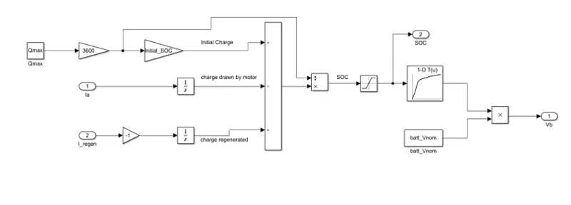
• Fig : Battery Model Subsystem

C. Transmission and Road Load Force Subsystem

A fixed Transmission ratio is considered whose model is as shown in Fig 4. The equations for transmission is given by

ω_w=ω_m/G_r  
T_m=T_w/G_r                                                               

eq (3.1)

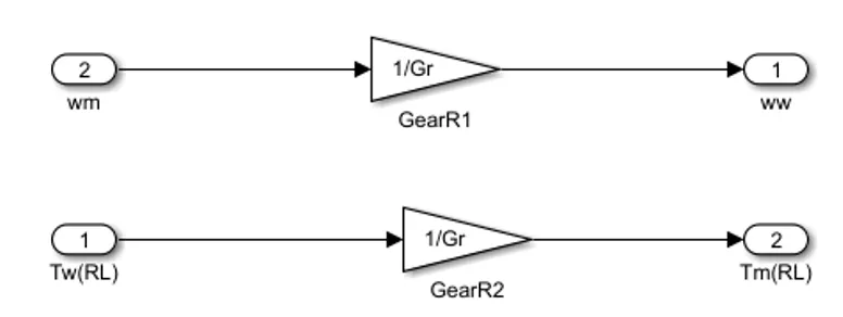
• Fig : Transmission subsystem

A vehicle's movement is governed by all the forces acting on it. The force that enables the vehicle to propel forward is called Tractive Effort. This force is due to the contact between the wheel of the vehicle on the road. The resistance forces encountered by a vehicle are:

• Rolling resistance force

Rolling resistance is the combination of forces that work against the forward motion of the vehicle. The weight of the vehicle, gravity and inertia, the amount of friction between the tires and the road surface, and air drag all play a part. When you coast a vehicle, rolling resistance is what slows down the vehicle. The more rolling resistance, the more power it takes to propel a vehicle.

 F_r=M_V×g×f_r×cos⁡∝ 

(3.2)

• Aerodynamic drag force

Any vehicle traveling at a speed in air encounters a force resisting its motion.

  F_a=0.5×rho×A_f×C_d×V^2                  

(3.3)

• Gradient resistance / Uphill drag force

When the vehicle travels uphill, a component of its weight works in a direction opposite to its motion. If some energy is not supplied to overcome this backward force, then the vehicle would slow down, stall and roll backward. If the vehicle is trading uphill at a slope of θ, then the weight of the vehicle, W has two components: one perpendicular to the road surface and the other along the road surface.

F_g=M_V×g×sin⁡∝                                    

(3.4)

The overall Road Load Force is given by

F_t=F_r+F_a+F_g+F_xf+F_xr                            

(3.5)

The net Road Load Force is sent to the motor module through the transmission to determine the acceleration is represented in Fig .

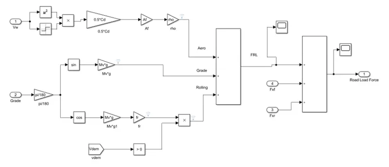
• Fig : Road Load Force Subsystem

D. Regenerative Current Monitor

This is a crucial subsystem that is used to monitor the maximum current entering the battery during regeneration. Similar to discharging the charging current entering the battery also has to be maintained within a certain current rating and to maintain the SOC of the battery. As shown in Fig 6 importance of this subsystem is that when SOC is greater than 80% then the regenerative current is discharged to avoid overcharging of the battery.

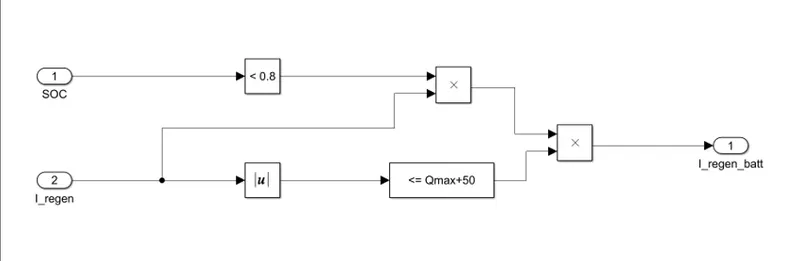
• Fig : Regenerative Current Monitor Subsystem

E. DC-DC Converter

This module lies between the Motor and the Battery. In this paper, the converter is simply modeled like a gearbox modeled as in Fig . DC-DC Converter supplied armature current to the motor at a lower potential by multiplying the current, while supplies the regenerated current to a higher potential battery the current is decreased.

〖Power〗_battery=〖Power〗_motor
I_b×V_b=I_m×V_m 

(4.1)

The converters do not operate at 100% efficiency. Accounting for 20% power loss, 80% converter efficiency is considered.

I_b×V_b×Conversion efficiency=I_m×V_m

(4.2)

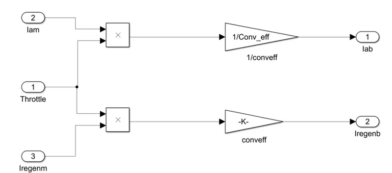
• Fig : DC-DC Converter Subsystem

F. Brake Subsystem

Modeling the distribution of brake forces between the front wheel (70%) and the rear wheel (30%) is shown in Fig .

F_(brake front)=(0.7×max⁡_brakeT)/r               

F_(brake rare)=(0.3×max⁡_brakeT)/r

(5.1)

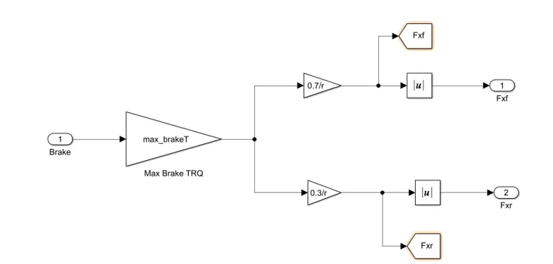
• Fig : Brake Subsystem

G. PID Controller Subsystem

PID controller is one of the simplest and efficient controllers used to optimize the results. The actual velocity is compared with demanded velocity to generate an error signal given to the PID Controller is shown in Fig . Switches are used to send the positive signals as the throttle command and negative signals as the brake command.

u(t)=K_p×e(t)+K_i×∫▒〖e(t)〗+K_d×(d(e(t)))/dt     

e(t)=v_dem-(v_act×3600)/1600                                           

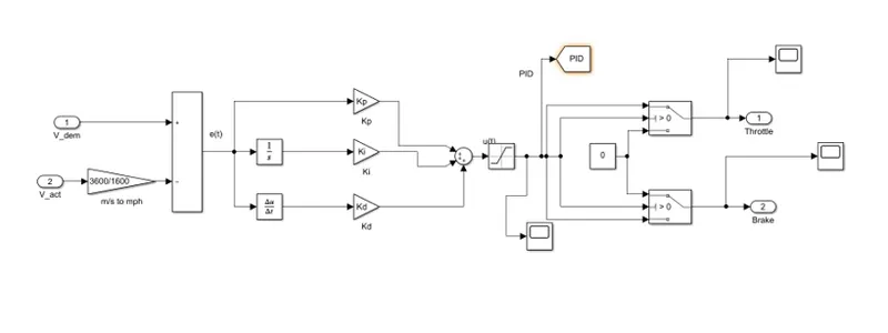
• Fig : PID Controller Subsystem

H. Overall Integrated Vehicle Design

All the necessary connections between different subsystems are made. Here, the velocity of the vehicle is assumed to be a product of the angular velocity of the wheel with its corresponding radius.

V_w= ω_(w )×r   

(7.1)

The throttle and brake signals are taken from the PID controller and are given to DC-DC Converter and Brake Actuators respectively as presented in Fig. Depending on the tests conducted the demanded velocity can be a drive cycle or a step signal.

A switch is built which stops the simulation once the SOC falls to 20%. Different scopes are used to compare actual and demanded velocity, to observe and torque, speed, current of the motor, and to measure the power consumed by the vehicle.

The electric vehicle is modeled using the basic equations. The DC motor supplies power to the wheels through the transmission unit. The vehicle's interaction with the environment is modeled in terms of gradient, acceleration, aerodynamic, and rolling resistance forces in the Road Load subsystem to Motor Subsystem through the transmission subsystem whose output is vehicle speed. The difference between the vehicle speed and the demanded speed given by the drive cycle is given as the input to the PID controller subsystem. This acts as a driver, reducing the error between the desired speed and actual speed by applying throttle or brake signals. The battery subsystem is the source of power in the vehicle. This supplies the motor current at a given voltage to overcome the resistances and achieve the velocity. When the vehicle slows down, the motor acts as a generator and supplies the current to the battery. The regeneration current monitor ensures that the battery does not overcharge. The DC-DC converter acts as a bridge between higher voltage battery and lower voltage motor thus conserving power.

Experimental Results

The tests provide a good characterization of the vehicle performance, aid in simulating a variety of real-life scenarios without increasing cost or time and help us to determine the average energy consumption for different drive cycles.

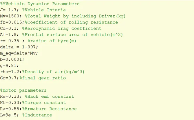
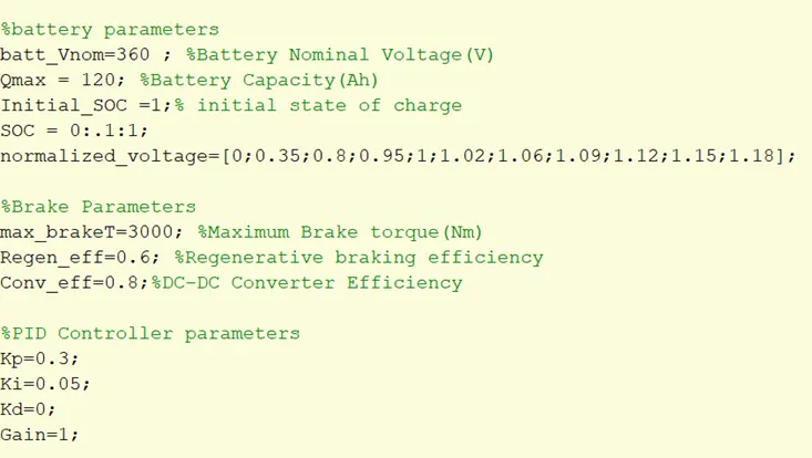
This paper takes the vehicle parameters of the BMW i3 electric vehicle as tabulated in Table 1. Table 2 represents BMWi3 performance parameters to compare the results of the model.

• BMW i3 Vehicle Parameters

Sl No.	BMW i3 Parameters	Values
1	Battery Nominal Voltage	360V
2	Battery Capacity	120Ah
3	Battery Total Energy	42.2kWh
4	Motor Maximum Power	125kW
5	Motor Torque	250Nm
6	Gear Ratio	9.665:1
7	Kerb Weight	1345kg
8	Radius of tire	0.35m

• BMWi3 Performance Parameters

Sl No	Parameters	Values
1	Acceleration	0-100mph in 7.2 secs
2	Top Speed	93mph
3	Range on EPA Drive Cycle	240km

A. Acceleration And Maximum Velocity Test

A step block whose final value is chosen to be 100 is connected as the demanded velocity input for PID Controller Subsystem.

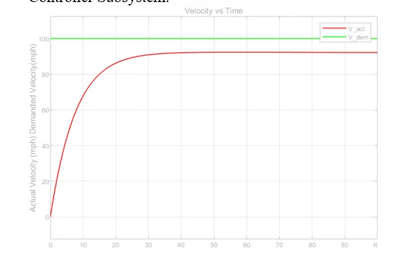
• Fig : Actual vs demanded velocity
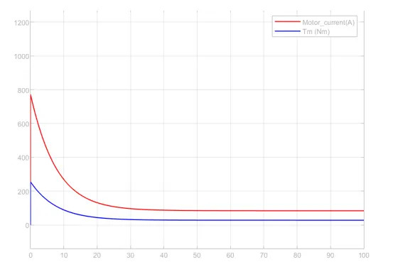
• Fig : Current drawn and torque output
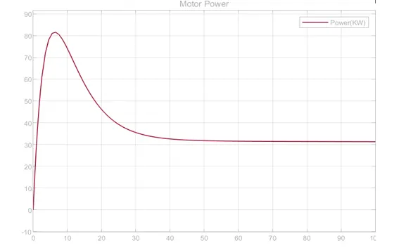
• Fig : Power required during acceleration

• Comparison of Performance Parameters

Sl. No	Parameter	BMW i3	Simulink Model
1	Acceleration Time	7.2 secs	8secs
2	Speed	93mph	92.5mph
3	Power for acceleration	125kW	81kW

The initial current can be observed from Fig to be approximately 772A since during starting the speed is zero hence back emf is zero. Therefore, the motor voltage applied across small resistance tends to give a large current. It can be seen that the torque decreases gradually as the speed increases and attains a value of 40Nm. Table 3 represents the comparison of performance parameters of the BMWi3 vehicle with the Simulink model.

B. Grade Test

Gradeability is defined as the highest grade a vehicle can ascend maintaining a particular speed. The power rating increases as the grade increases. Hence plays a crucial role in deciding the performance of the vehicle.

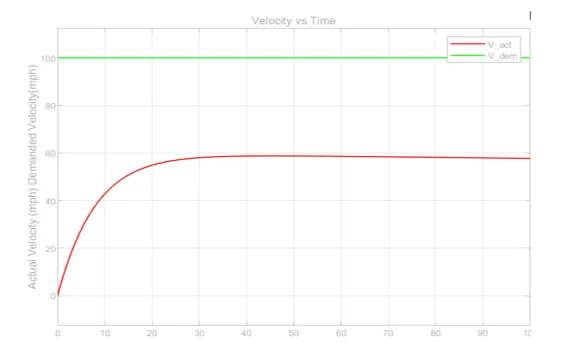
By setting the value of grade to 10 which is equivalent to 45 degrees’ inclination, we can see from Fig that the actual velocity does not follow the demanded velocity as the difference is more.

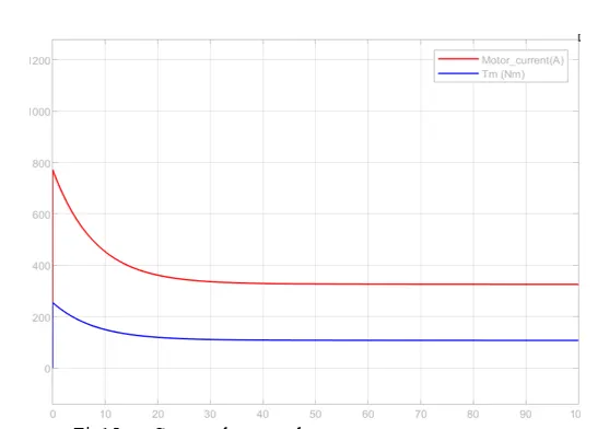
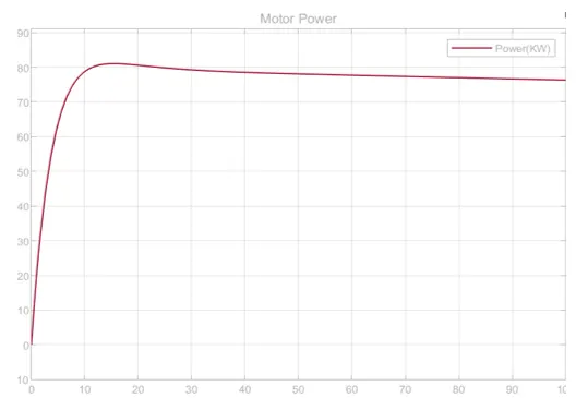
The steady-state current is close to 325 A as observed in Fig and torque is 107Nm. As the weight of the vehicle is adding resistance force the power required by the motor is shown in Fig

• Fig: Actual vs demanded velocity

• Fig : Current drawn and torque output

• Fig: Power required at 10 grade

C. Drive Cycle Tests

Drive Cycles are an important instrument in the development of new vehicles and for the evaluation of vehicle characteristics like energy consumption and emissions. By running drive cycle tests the characteristics of an electric vehicle can be assessed for optimizing components.

Drive Cycle test is performed to analyze battery state and energy consumption in EVs and to simulate vehicle model prior to the actual development.

• US06 Drive Cycle

It is a high acceleration aggressive driving schedule that is identified as “Supplemental FTP”.

The average speed of the US06 drive cycle is 48.37 mph with a range of 8.01 miles in 596 secs.

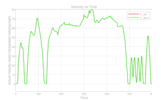
Fig: US06 drive cycle and actual vehicle speed comparison

• 
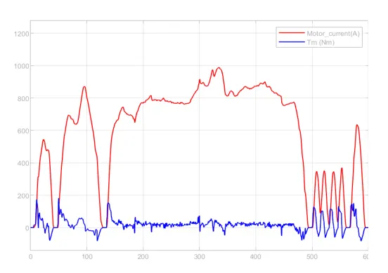
• Fig : Torque and current demanded on US06 Drive Cycle
• 
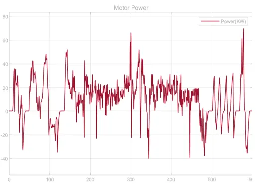
• Fig: Power demanded by the US06 Drive Cycle

The average speed of 48.37 is successfully achieved by the model. Due to the aggressive acceleration, the peak current is 553 A with a peak torque of 182 Nm and a maximum power of 69KW.

• UDDS Drive Cycle

The Urban Dynamometer Driving Schedule is commonly called the "city test" as it represents the city driving conditions. Used for light-duty vehicle testing.

The UDDS Drive cycle has an average speed of 19.59 mph with a range of 7.42miles in 1369 seconds.

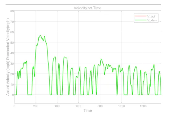
Fig: UDDS Drive Cycle and actual vehicle speed comparison

• 
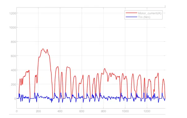
• Fig : Torque and current demanded on UDDS Drive Cycle
• 
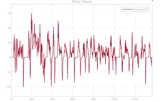
• Fig: Power demanded by the UDDS Drive Cycle

UDDS has rapid speed changes and is a more aggressive drive cycle that draws a maximum current of 239 A and demands a torque of 78Nm with a maximum power of 30 KW.

• EPA Drive Cycle

The EPA Drive Cycle represents highway driving with an average speed of 48.3 mph with a range of 10.26 miles in 765 seconds.

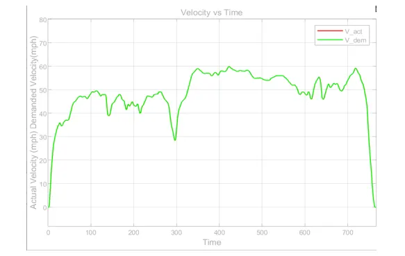
• Fig: EPA Drive Cycle and actual velocity speed comparison

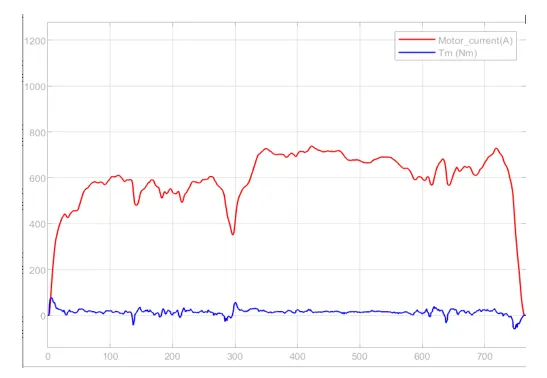
Fig : Torque and current demanded on EPA drive cycle

• 
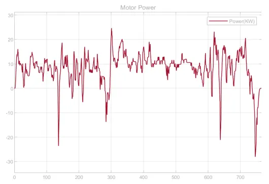
• Fig: Power demanded by the EPA Drive cycle

This test is mainly conducted for the fuel economy test of light-duty vehicles. It draws a maximum current of 230A. The maximum torque is 76Nm with a maximum power of 24KW.

• WLTP3 Drive Cycle

This represents a more dynamic velocity profile, consists of quicker accelerations and small brakes with a maximum acceleration of 1.6m/s², a maximum speed of 81 mph, and a range of 14.3 miles in 1800 seconds.

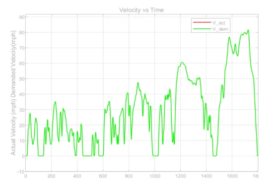
• Fig: WLTP3 Drive cycle and actual vehicle speed comparison

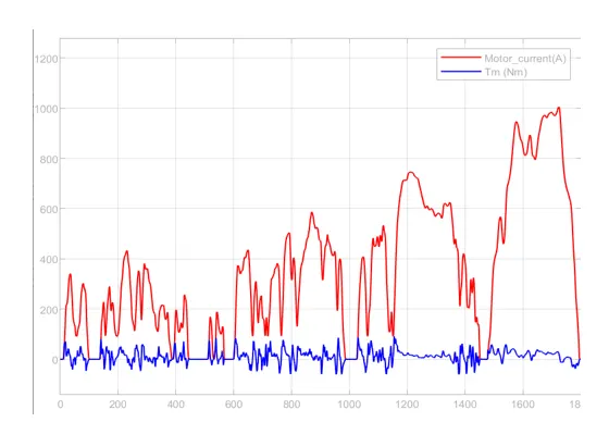
Fig : Torque and current demanded on WLTP3 Drive Cycle

• 
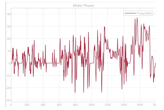
• Fig : Power demanded by the WLTP3 Drive cycle

This cycle is mainly divided into 4 sub-parts, each of them having separate maximum speeds- Low: 35.1mph, Medium: 47.6mph, High: 60.5mph, Extra-high: 81.6mph. These phases simulate urban, suburban, rural, and highway scenarios. This cycle draws a maximum current of 275A, a maximum torque of 90Nm, and demands a power of 37KW during a high-speed range.

The integrated electric vehicle model simulated for analyzing the performance characterization of an electric vehicle was compared with the BMW i3 to compare closely the performance of the vehicle. This model described the performance requirements concerning top speed, time taken for acceleration to 60mph, and the performance with a 45-degree gradient. Different drive cycle tests show the performance of the vehicle model designed. Based on the results, it can be concluded that the proposed model can be used to estimate the performance of the electric vehicle by knowing the vehicle parameters. This model is reliable as it gives precise results for most of the parameters which are close to the actual vehicle design. Further, the same model can be tested by changing the EV motor subsystem block with BLDC/PMSM motor model to see the improvements concerning acceleration and grading. With modifications to this model, the range of the vehicle can be calculated. Also, this model can be converted to series or parallel hybrid by including the engine and using engine and motor control strategies.