Final Project: Design of an Electric Vehicle

Introduction :

An Electric Vehicle , also known as Battery Electric Vehicle(BEV) are fully electric vehicles that runs on battery power, which is charged using electricity grid. EV’s are also called zero emission vehicles as they do not produce any exhaust emissions like the traditional vehicles. With growing issue of global warming and reduction of non-renewable fuels, EV’s are the technology to look for.

New technology like high-capacity lithium type battery will be a major energy source for the propulsion of electric vehicles. At present, with the new technologies, some manufacturer has launched its products which are Tesla, Chevy Bolt EV and Nissan leaf which are fully electric battery-based car.

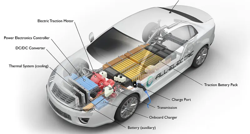
The components of electric vehicle are :

1. Auxiliary Battery: In an electric drive vehicle, the auxiliary battery provides electricity to power vehicle accessories.
2. Traction Battery Pack: Traction battery pack is also known as Electric Vehicle Battery (EVB) which is used to store the energy. This energy facilitates the propulsion power for the vehicle. Some examples of traction battery energy storage are -

• Lithium-Ion
• Nickel-Metal Hydride
• Lead-Acid
• Ultra-Capacitors

3. DC/DC Converter: It is a power-electronic converter circuit, used to convert high voltage DC power from the traction battery pack to a lower-voltage DC power. The converted power is used to run the vehicle accessories and it is also used to recharge the auxiliary battery.
4. Electric Traction Motor: In an EV, one of the most important components is electric traction motor. It provides power to the wheels to move and also helps in regenerating energy. Traction motor can be a DC motor or AC induction motor,
5. Onboard charger: It is the device that takes the incoming AC supply via the charge port and converts it to DC power for charging the traction battery. It monitors battery characteristics such as voltage, current, temperature, and state of charge while charging the pack.
6. Power electronics controller: This unit manages the flow of electrical energy delivered by the traction battery, controlling the speed of the electric traction motor and the torque it produces.
7. Charge port: The charge port enables the vehicle to connect to an external power supply (Electrical Grid) in order to charge the traction battery pack.
8. Thermal system (cooling): This system maintains a proper operating temperature range of the electric motor, power electronics, and other components.

OBJECTIVE FOR DESIGNING AN EV:

1. To make a simple & low run time vehicle model using individual component models.
2. To check out performance parameters: Speed, SOC, Current etc with various drive cycles.
3. To play with: Motor power, Vehicle body (Rolling resistance, Air drag, Weight) inputs.
4. To know MATLAB models & their configuration to match with actual vehicle.

BLOCK DIAGRAM:

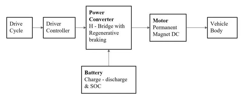
Modelling of EV using Simulink :

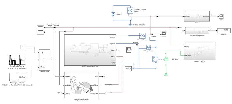
The above figure shows the complete model of an Electric Vehicle. It comprises of 4 subsystems like – power controller, vehicle body, battery SOC and distance calculation. The components DC Motor and Battery are in the open for quick access. The breakdown of each components is discussed below-

A.) Vehicle body Subsystem :

This subsystem represents the body of the vehicle along with gear box and wheels.

The block diagram of this subsystem is given below-

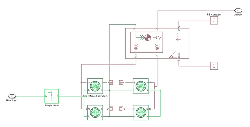
• Tires: As we are designing a 4-wheeler EV so we require 4 tires. The tire(magic formula) block is here having 4 ports H,S,N and A. H represents Hub, S as Tire slip, N as Normal Force and A as Axle connection.
• Vehicle Body: - This block represents a two-axle vehicle body in longitudinal motion. It accounts for body mass, aerodynamic drag, road incline, and weight distribution between axles due to acceleration and road profile.

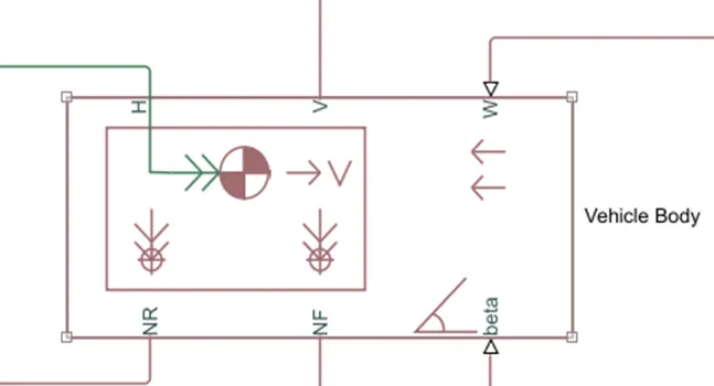
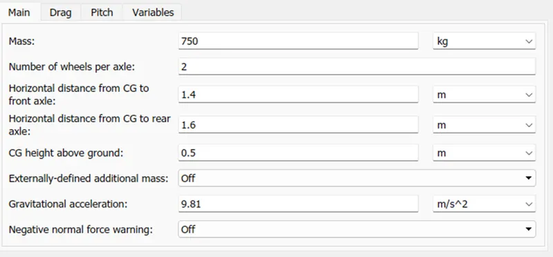
Connection H is the mechanical translational conserving port associated with the horizontal motion of the vehicle body. The resulting traction motion developed by tires should be connected to this port. Connections V, NF, and NR are physical signal output ports for vehicle velocity and front and rear normal wheel forces, respectively. Wheel forces are considered positive if acting downwards. Connections W and beta are physical signal input ports corresponding to headwind speed and road inclination angle, respectively. If variable mass is modelled, the physical signal input ports CG and M are exposed. CG accepts a two- element vector representing the x and y distance offsets from vehicle CG to additional load mass CG. M represents the additional mass. If both variable mass and pitch dynamics are included, the physical signal port J accepts the inertia of the additional mass about its own CG.

For our simulation this block is configured as follows-

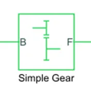
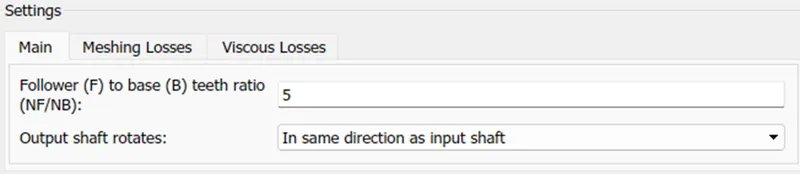
• Simple Gear: - This block is used to represents a fixed-ratio gear or gear box. No inertia or compliance is modelled in this block. It has the option to include gear meshing and viscous bearing losses. Connections B (base) and F (follower) are mechanical rotational conserving ports. Specify the relation between base and follower rotation directions with the Output shaft rotates parameter. Optionally include thermal effects and expose thermal conserving port H by setting Friction model to a temperature-dependent setting.

Connections and Summary:

Here, we first set the tires which will be operated through gear & vehicle body from motor. In this case it’s a rear wheel drive. Then, we setup the vehicle body which will represent all the weights of the car and connects tires and a input is put open for velocity which will come from drive cycle later. Then we added simple gear which will help to move vehicle with the help of tires. The input to the gearbox which will come from shaft of the motor.

Hence, we are ready with the base of our EV.

B). Power Controller Subsystem:

The power controller subsystem is the heart of the EV. The block diagram shown below-

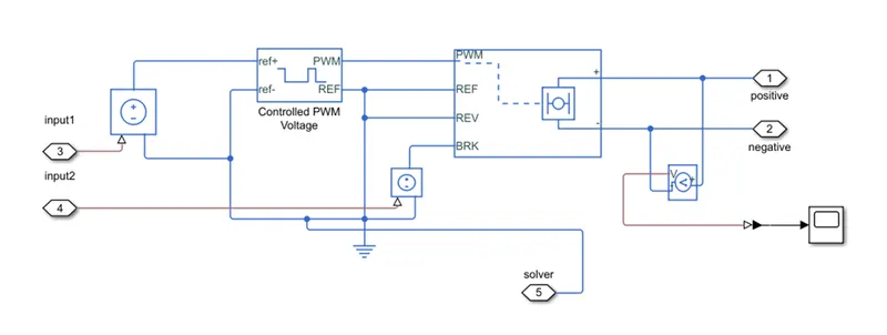
The above subsystem contains following components: -

• H-bridge: This block represents an H-bridge motor drive. The block can be driven by the Controlled PWM Voltage block in PWM or Averaged mode. In PWM mode, the motor is powered if the PWM port voltage is above the Enable threshold voltage. In Averaged mode, the PWM port voltage divided by the PWM signal amplitude parameter defines the ratio of the on-time to the PWM period. Using this ratio and assumptions about the load, the block applies an average voltage to the load that achieves the correct average load current. The Simulation mode parameter value must be the same for the Controlled PWM Voltage and H-Bridge blocks. In simple words it’s a 4 switch converter. And the block is configured as-

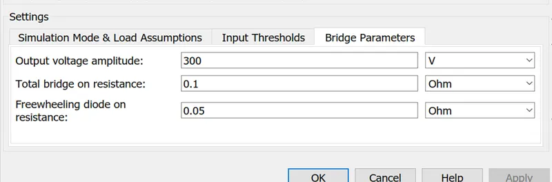
• Controlled PWM voltage: This block creates a Pulse-Width Modulated (PWM) voltage across the PWM and REF ports. The output voltage is zero when the pulse is low, and is equal to the Output voltage amplitude parameter when high. Duty cycle is set by the input value.

Summary of the subsystem:

The H-bridge is used due to the four inputs from PWM generators, REV, REF and braking. The positive and negative terminal is connected to DC motor. A voltage sensor is attached across the terminals. The PWM controlled voltage control is used for input to H-bridge. Hence, in this subsystem we constructed the control system of our vehicle, where the two inputs are coming from longitudinal driver which commands control and both the components operate accordingly.

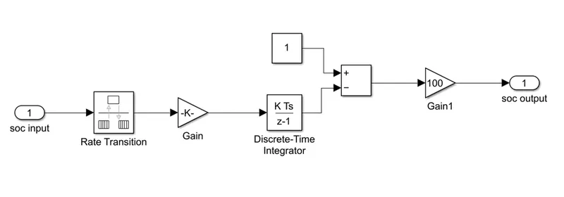
C). SOC Subsystem:

This subsystem is made to observe the battery dissipation of the vehicle when it will be in running and shows the % of battery left. It contains of rate transition and discrete time integrator which converts and help in exchange of signals.

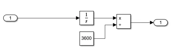
D).DISTANCE CALCULATION:

This subsystem is made as a display to see the distance travelled by the vehicle. It contains an integrator, which helps to show the distance in kms when 3600 constant is multiplied to it.

So, up till now we constructed all the subsystems for the model, now we will move to the Battery pack and the Motor configuration.

Here we have considered a simple DC motor with the following configurations -

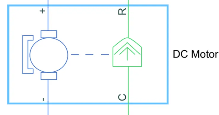
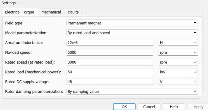
This block represents the electrical and torque characteristics of a DC motor. The block assumes that no electromagnetic energy is lost, and hence the back-emf and torque constants have the same numerical value when in SI units. Motor parameters can either be specified directly, or derived from no-load speed and stall torque. If no information is available on armature inductance, this parameter can be set to some small non-zero value. When a positive current flows from the electrical + to - ports, a positive torque acts from the mechanical C to R ports. Motor torque direction can be changed by altering the sign of the back-emf or torque constants.

It takes the input command from motor controller and delivers to transmission system. And for the time when vehicle gets brake it will work as generator and charge the battery for that moment due to regenerative braking.

Now, comes the battery pack. We are using a simple battery for quick simulation, with following parameters--

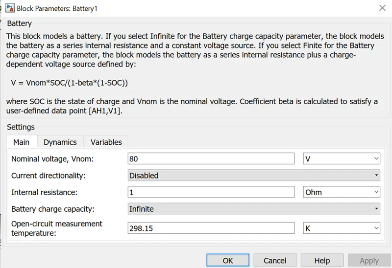
LONGITUDINAL DRIVER: - It takes the input from velocity input for the drive cycles and give commands to motor controller so that it handles motor speed according to given drive cycles. But it is very difficult to maintain the same drive cycle as commanded.

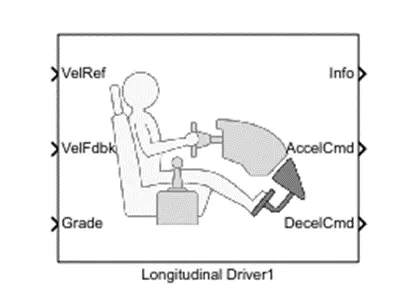
So, we have included almost every important part of the model, but the input, which is most important for driving a vehicle.

VELOCITY INPUT: It is the multi-port input which Pass through the input signals corresponding to the truncated value of the first input. The inputs are numbered top to bottom (or left to right). The first input port is the control port. The other input ports are data ports. And we can give as many input as we want.

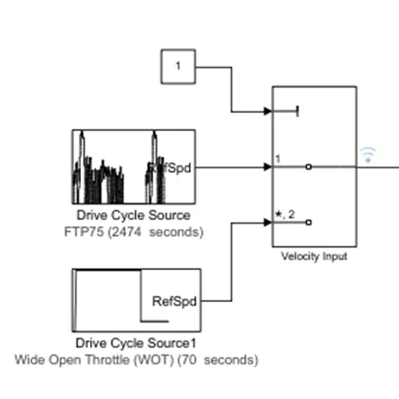
Here, we have given two drive cycles, if we want, we can even provide our own cycles with the help of self-made spreadsheet file attaching to multi-port switch.

WORKING:

Input Drive Cycle is given as soon as motor gets excited. The desired input from user is given to Velocity Input (i.e., to multiport switch) and it delivered cycles are been recorded for the comparison of initial input cycle and final output drive cycle. The same is been inputted to Longitudinal Driver which decodes the command and converts it to machine language and moves ahead to Motor Controller, (the commands are been executed with the help of Controlled PWM Voltage), which generates the pulses and H-Bridge which takes the multiple input and with the help of voltage and current sensors delivers the command signal to Motor.

According to the signals, the current and voltage fluctuation is noted. Then Controlled Motor, signals to transmission system (which is the real practical part), where a simple gear is attached to the wheels(tires) offers acceleration, de-acceleration, braking and reverse motoring and thus, accordingly vehicle body works.

The final velocity is been recorded and later to be compared with inputted one.

Simultaneously, battery performance is also recorded for calculating the efficiency of the vehicle over the journey period. Now, let’s see the results.

RESULTS:

Input Drive cycle vs Resultant drive cycle: The model is simulated for FTP75 drive cycle which is 2474 seconds long , the results are fetched as below-

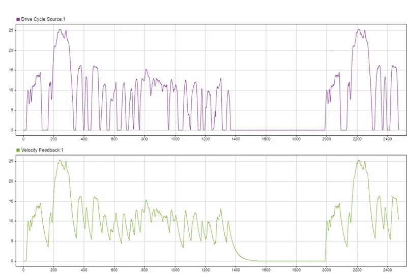
The above figure shows the plot both the drive cycles, the first plot is the input signal and the second is the final output.

From observing the plot, it noted that -

• Both signals are almost same while acceleration command is given.
• While deacceleration also the output almost tried to copy the input signal, but it is not matched 100%.
• When a sudden braking input is applied to the model it is not replicating to the input.

The sudden braking input could not be replicated as it is dangerous and more or less impossible to stop the running car running at certain velocity as it acquires certain kinetic energy and work done starts.

Output Current and voltage:

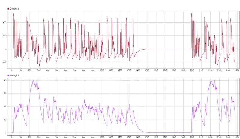
We can see a huge fluctuation is occurred during the drive cycle, while the vehicle experiences acceleration, deacceleration and braking. For some time vehicle seen to be running in constant speed and at rest in middle of journey too.

SOC and Distance:

As the vehicle is simulated, it is considered to have 100% SOC at the beginning. The data collected after the simulation is given below.

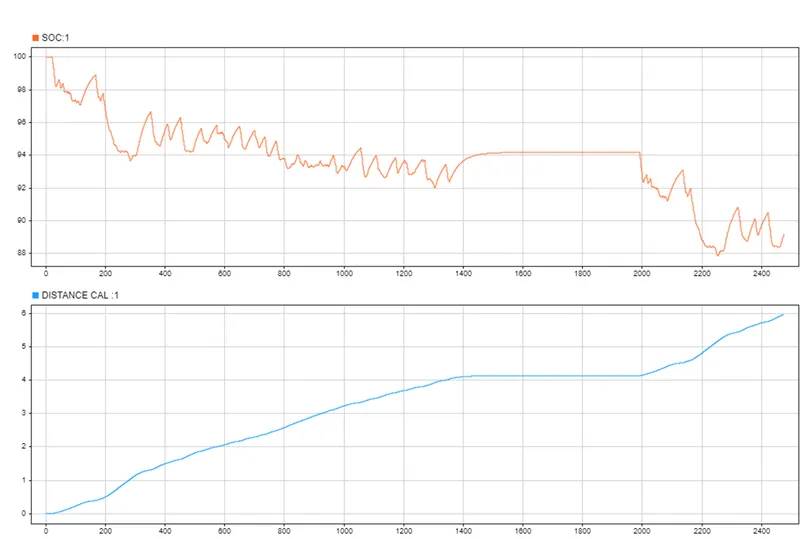
Here, we can see after the end of the drive cycle, the final soc of the vehicle is around 88%. The vehicle travelled a distance of around 6 km and for that purpose, it only used around 12% of the battery charge. Because of the regenerative braking it also gained some energy back. This, improves the efficiency and also reduces the cost of the journey.

CONCLUSION:

So building a vehicle model from scratch gives a scope to learn about the processes and equipments that makes a vehicle run in the roads. This model is a simpler one. With the use of more depth, this model can be calibrated to real vehicles. The model built is tested in against the FTP drive cycle. More testing can be done with different drive cycles. If we want increase the performance , that also can be done by changing Motor and battery parameters.

So, as a whole the concept of Electric vehicle is evolving and in coming days technology will improve and clearly surpass the ICE vehicle in the roads.