Final Project: Design of an Electric Vehicle

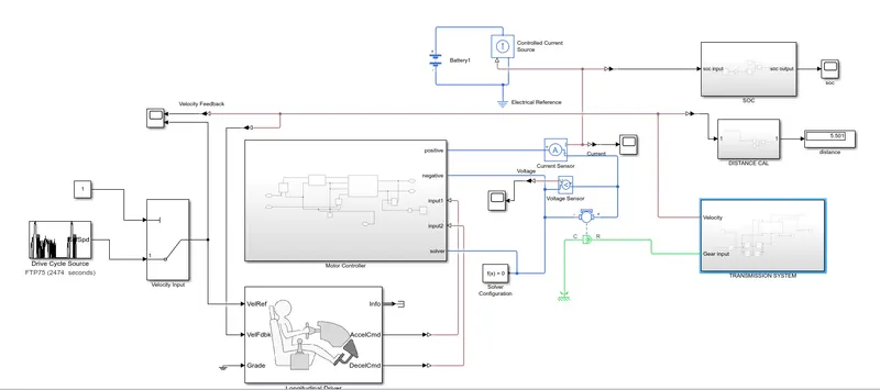
Create a MATLAB model of electric car which uses a battery and a DC motor. Choose suitable blocks from Powertrain block set.

Prepare a report about your model including following:

Objectives:

1. System level configurations

2. Model parameters

3. Results

4. Conclusion

MATLAB model of electric car:

System Level Configurations:

1. Drive cycle
2. Multiport switch
3. Longitudinal driver block
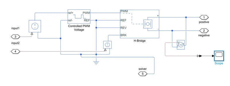
4. PWM controller
5. H Bridge
6. Controlled Voltage source
7. Controlled current source
8. Voltage sensor
9. current sensor
10. dispaly
11. constant block
12. Scope
13. DC Motor
14. Battery
15. Simple gear block
16. tire (magic formula)
17. Integrator

Subsystems:

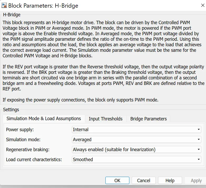
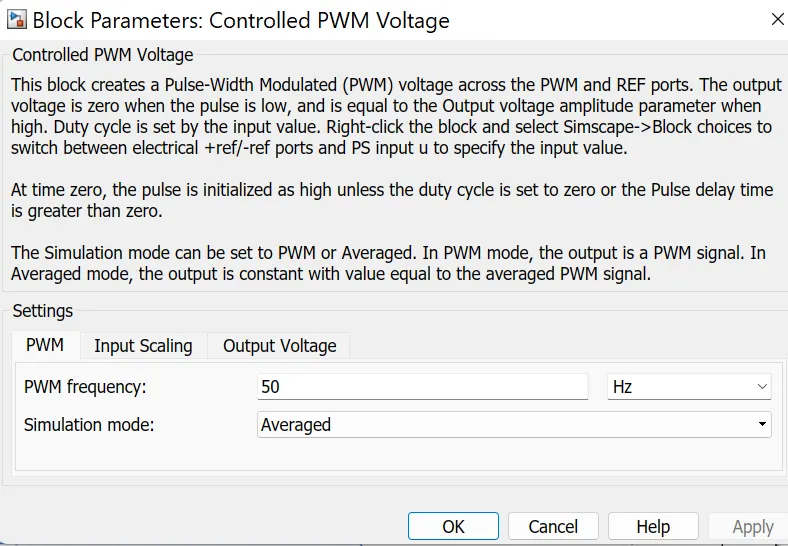
1. Motor Cotroller Subsystem
2. Transmission Subsystem
3. SOC Subsystem
4. Distance calculation

All the above blocks are connected as below to model an electric vehicle:

MODEL PARAMETERS:

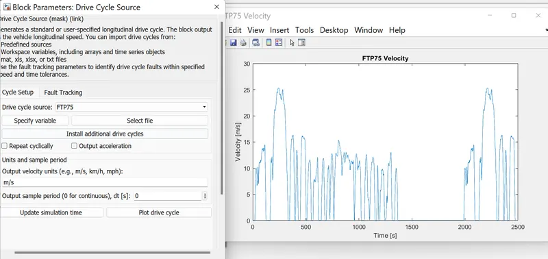
Drive cycle Block:

Description

The Drive Cycle Source block generates a standard or user-specified longitudinal drive cycle. The block output is the specified vehicle longitudinal speed,

which you can use to:

• Predict the engine torque and fuel consumption that a vehicle requires to achieve desired speed and acceleration for a given gear shift reference.
• Produce realistic velocity and shift references for closed loop acceleration and braking commands for vehicle control and plant models.
• Study, tune, and optimize vehicle control, system performance, and system robustness over multiple drive cycles.
• Identify the faults within tolerances specified by standardized tests, including:
  
  
• EPA dynamometer driving schedules
• Worldwide Harmonised Light Vehicle Test Procedure (WLTP) laboratory tests

For the drive cycles, you can use:

• Drive cycles from predefined sources. By default, the block includes the FTP–75 drive cycle. To install additional drive cycles from a support package.
• Workspace variables that define your own drive cycles.
• .mat, .xls, .xlsx, or .txt files.
• Wide open throttle (WOT) parameters, including initial and nominal reference speed, deceleration start time, and final reference speed.

To achieve the goals listed in the table, use the specified Drive Cycle Source block parameter options

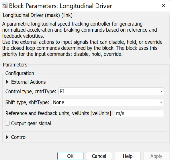
Longitudinal Driver Block:

Description:

The Longitudinal Driver block implements a longitudinal speed-tracking controller. Based on reference and feedback velocities,

the block generates normalized acceleration and braking commands that can vary from 0 through 1. You can use the block to model

the dynamic response of a driver or to generate the commands necessary to track a longitudinal drive cycle

Motor controller Subsystem:

DC MOTOR:

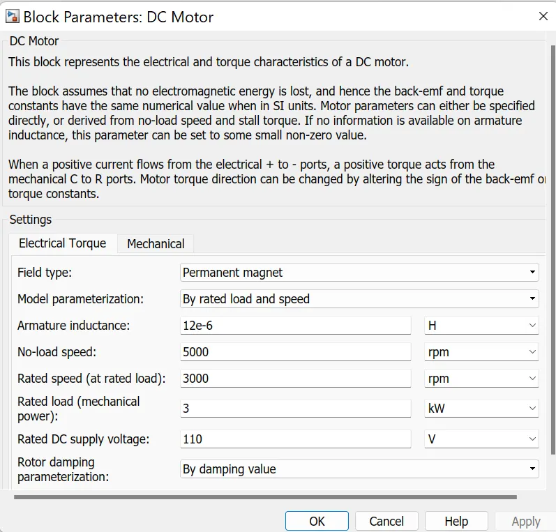
Description

The DC Motor block represents the electrical and torque characteristics of a DC motor using the following equivalent circuit model:

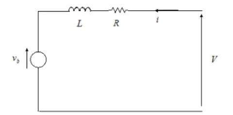
You specify the equivalent circuit parameters for this model when you set the Model parameterization parameter'

to By equivalent circuit parameters. The resistor R corresponds to the resistance you specify in the Armature resistance parameter.

The inductor L corresponds to the inductance you specify in the Armature inductance parameter.

You can specify how to generate the magnetic field of the DC motor by setting the Field type parameter to the desired option.

The permanent magnets in the motor induce the following back emf vb in the armature:

Transmission Subsystem:

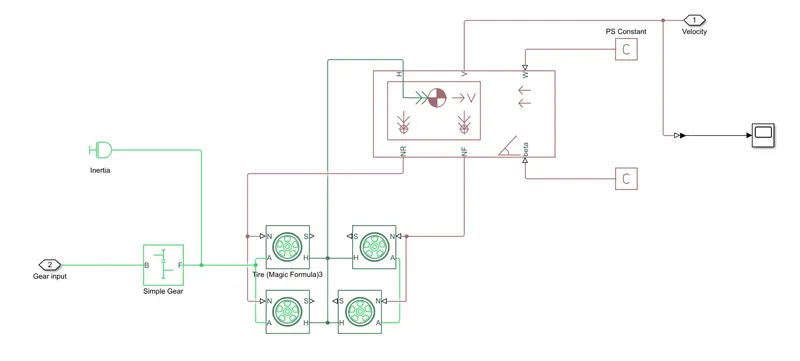
Vehicle Body Description:

• The Vehicle Body block represents a two-axle vehicle body in longitudinal motion. The vehicle can have the same

or a different number of wheels on each axle. For example, two wheels on the front axle and one wheel on the rear axle.

The vehicle wheels are assumed identical in size. The vehicle can also have a center of gravity (CG) that is at or below the plane of travel.

The block accounts for body mass, aerodynamic drag, road incline, and weight distribution between axles due to acceleration

and road profile. Optionally include pitch and suspension dynamics. The vehicle does not move vertically relative to the ground.

The block has an option to include an externally-defined mass and an externally-defined inertia. The mass, inertia, and center of

gravity of the vehicle body can vary over the course of simulation in response to system changes.

Tire (Magic Formula):

Description

• The Tire (Magic Formula) block models a tire with longitudinal behavior given by the Magic Formula ,

an empirical equation based on four fitting coefficients. The block can model tire dynamics under constant or variable pavement conditions.

The longitudinal direction of the tire is the same as its direction of motion as it rolls on pavement.

To increase the fidelity of the tire model, you can specify properties such as tire compliance, inertia, and rolling resistance.

However, these properties increase the complexity of the tire model and can slow down simulation. Consider ignoring tire

compliance and inertia if simulating the model in real time or if preparing the model for hardware-in-the-loop (HIL) simulation.

Simple Gear:

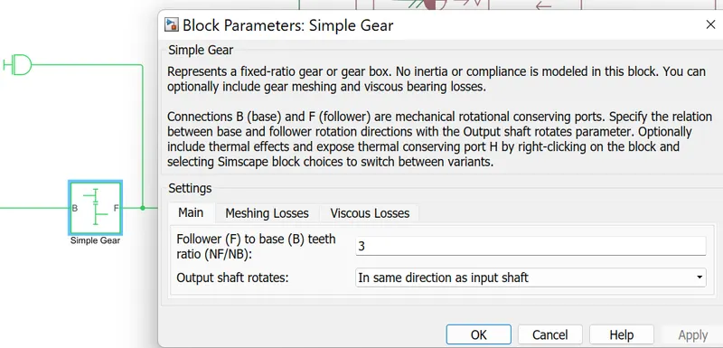
• This example shows a simple gear coupling two inertias (shafts). The gear ratio between the follower (F)

and base (B) is 2:1. Thus the angular velocity of the follower shaft is half the angular velocity of the base shaft.

The follower shaft torque is twice the base shaft torque.

An alternative to adding sensors to your model is to use Simscape data logging. This example has data logging enabled,

passing results to the workspace variable 'simlog_sdl_gear'. For example, entering 'plot(simlog_sdl_gear.Gear.B.w)' at the command

line plots the angular velocity at port B of the Gear block. See the Data Logging Example in the Simscape User Guide for further details.

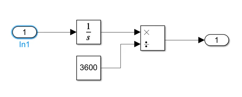
Distance calculation:

Armature Voltage Supply:

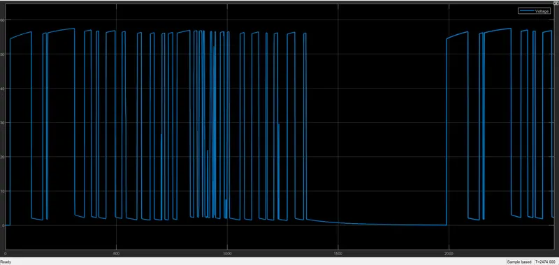
Graph Explanation:

1. The armature supply voltage is shown above.

2. It is in the range of 0 - 60V. As per the requirement of the drive cycle the voltage varies.

Armature Current:

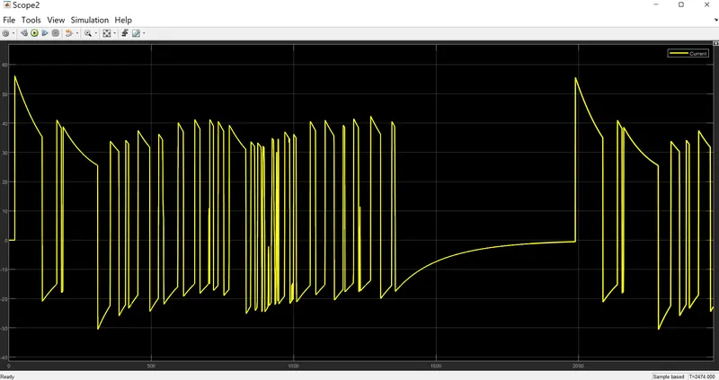
Graph Explanation:

1. The armature current of DC motor is shown in the above graph it varies in the of 55 to -30 amps.

2. Positive Voltage indicates the motoring mode of the motor.

3. Negative voltage indicates regenerative mode of the vehicle.

4.

Output:

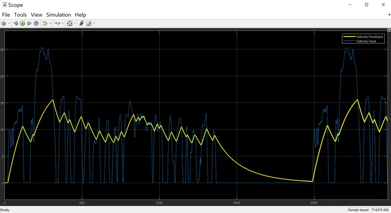
Graph Explanation:

1. Blue line is the drive cycle input.
2. Yellow line is the vehicle speed.
3. From the graph we can notice that vehicle is moving as per the drive cycle input.
4. I tried to minimise the sudden speed variations.

SOC of BATTERY:

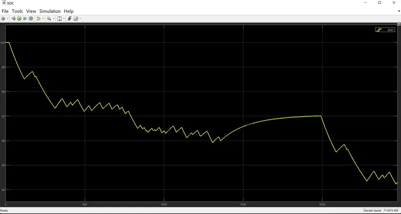
Graph Explanation:

1. SOC: State of charge of battery.
2. The battery is discharged upto 94%.
3. We can notice discharging and charging of the battery.
4. While discharging the vehicle is in acceleration mode
5. In charging mode the vehicle is in braking mode.

Output:

Distance Travelled by the vehicle:

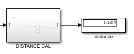
The total distance travelled by the vehicle is 5.501 Km that is shown in the Display block.

Conclusion:

1. Matlab model of electric vehicle is created and simulated.
2. The Results are explained briefly
3. Simulink model is attached.