Final Project: Design of an Electric Vehicle

Create a MATLAB model of an electric car that uses a battery and a DC motor. Choose suitable blocks from the Powertrain block set. Prepare a report about your model including the following:

Objectives:

1. System-level configurations

2. Model parameters

3. Results

4. Conclusion

Explanation

The basic theory of EV

An electric vehicle (EV) is one that operates on an electric motor, instead of an internal-combustion engine that generates power by burning a mix of fuel and gases. Therefore, a vehicle is seen as a possible replacement for current-generation automobiles, in order to address the issue of rising pollution, global warming, depleting natural resources, etc. Though the concept of electric vehicles has been around for a long time, it has drawn a considerable amount of interest in the past decade amid a rising carbon footprint and other environmental impacts of fuel-based vehicles.

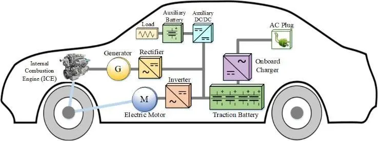
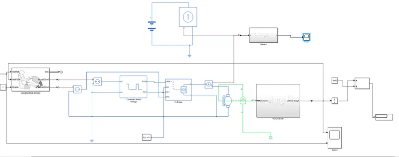
MATLAB model components of the EV has been explained below

Vehicle Body System

Tire (Magic Formula)

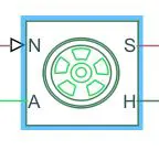
Represents the longitudinal behaviour of a highway tire characterized by the tire Magic Formula. The block is built from Tire-Road Interaction (Magic Formula) and Simscape Foundation Library Wheel and Axle blocks. Optionally, the effects of tire inertia, stiffness, and damping can be included.

Connection A is the mechanical rotational conserving port for the wheel axle. Connection H is the mechanical translational conserving port for the wheel hub through which the thrust developed by the tire is applied to the vehicle. Connection N is a physical signal input port that applies the normal force acting on the tire. The force is considered positive if it acts downwards. Connection S is a physical signal output port that reports the tire slip. Optionally expose physical signal port M by setting Parameterize by to Physical signal Magic Formula coefficients. Physical signal port M accepts a four-element vector corresponding to the B, C, D, and E Magic Formula coefficients.

The vehicle is assumed to be front axle is driven (4 wheels - 2 on each axle).
The wheels are modelled using simple Tire (Magic formula) Simulink blocks.

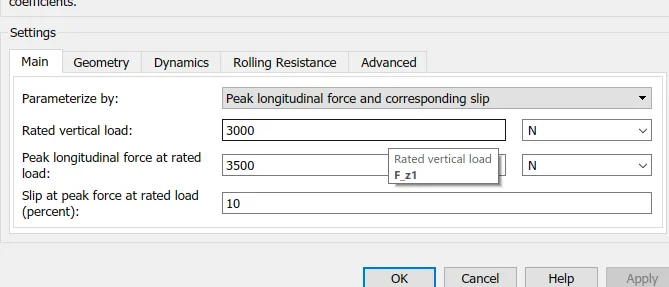
The tires are parameterized by Peak longitudinal force and corresponding slip
The other block parameters such as - rated vertical load, peak longitudinal force at rated load and slip at peak force at rated load - are kept with their default values.
The tire radius is given as 0.3 m
The tire inertia is kept as 1 kg-m^2
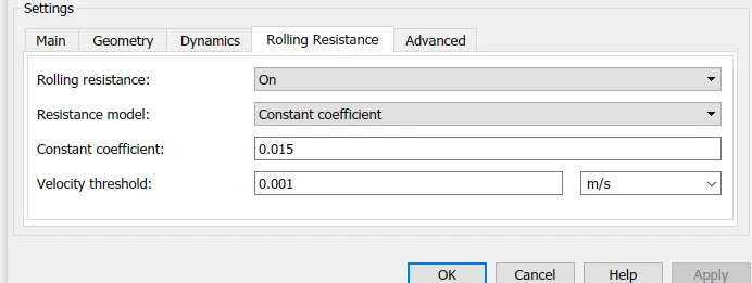
Also, the rolling resistance is given with a constant coefficient of 0.015

Vehical Body

This 2 axle (4 wheels) assembly is now connected to a Velocity Body simscape block.

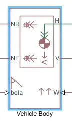
Represents a two-axle vehicle body in longitudinal motion. The block accounts for body mass, aerodynamic drag, road incline, and weight distribution between axles due to acceleration and road profile. The vehicle can have the same or a different number of wheels on each axle. Optionally include pitch and suspension dynamics or additional variable mass and inertia. The vehicle does not move vertically relative to the ground.

Connection H is the mechanical translational conserving port associated with the horizontal motion of the vehicle body. The resulting traction motion developed by tires should be connected to this port. Connections V, NF, and NR are physical signal output ports for vehicle velocity and front and rear normal wheel forces, respectively. Wheel forces are considered positive if acting downwards. Connections W and beta are physical signal input ports corresponding to headwind speed and road inclination angle, respectively. If the variable mass is modelled, the physical signal input ports CG and M are exposed. CG accepts a two-element vector representing the x and y distance offsets from vehicle CG to additional load mass CG. M represents the additional mass. If both variable mass and pitch dynamics are included, the physical signal port J accepts the inertia of the additional mass about its own CG.

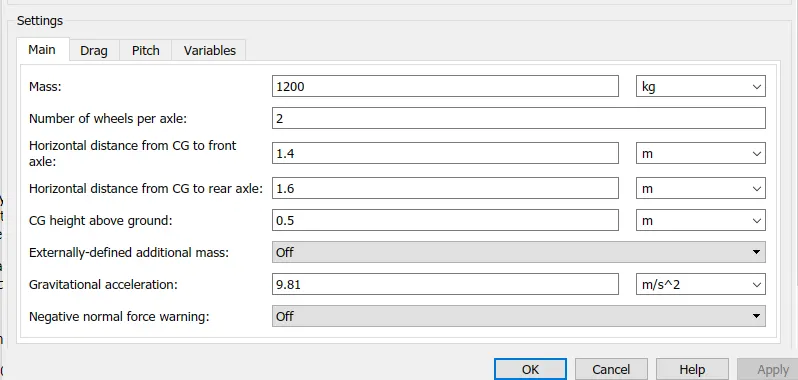
The gross weight is given to be 1200 kg
The geometric parameters of the vehicle are given as

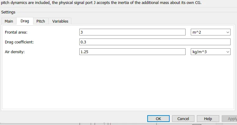
To account for proper drag force on the vehicle, the related parameters are kept as

The pitch dynamics for the vehicle are not considered for this simulation

The complete Vehical Body is shown below

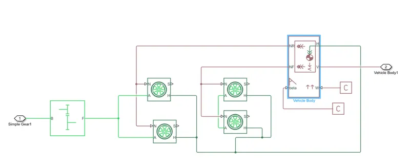
The input for this subsystem is taken as the Rotational speed of the motor. This input is fed to the front axle through a Simple Gear representing the Final Drive Ratio of 3.73
Here, the rotational direction of the output shaft is kept the same as that of the input shaft. Also, no meshing losses are considered for the simulation.

DC Motor

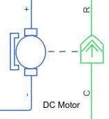
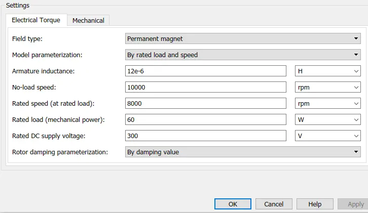
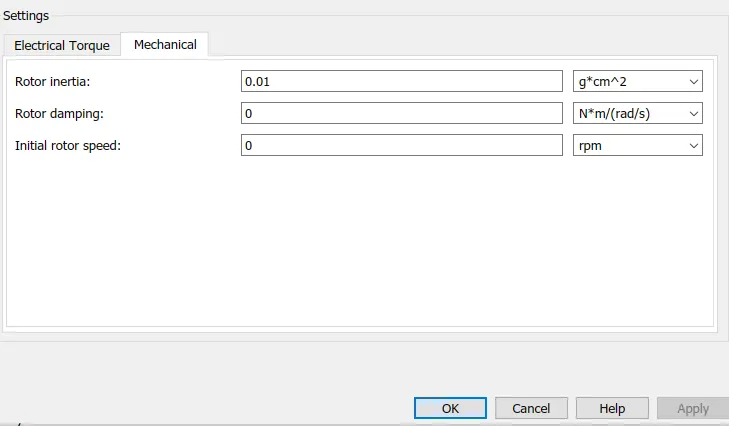
Here, the motor field type is kept as a Permanent magnet and the model parameterization is done by rated load and speed. The armature inductance and the mechanical parameters are given their default values.
All the other parameters are changed as shown below

The connection R represents the Rotor (rotational output) while the connection C is for the Casing (stationary).

Thus, the R port is connected to the input of the vehicle subsystem created earlier. The C port is connected to a mechanical rotational reference
The + and - terminals of the motor are connected to the motor controller. If these terminals are directly connected to a battery, the required DC motor will run on the rated capacity of the battery. This will eventually result in no control over the DC motor and the vehicle will run at top speed throughout the simulation.
Thus, a motor controller is very much needed.

Motor Controller circuit

This block represents an H-bridge motor drive. The block can be driven by the Controlled PWM Voltage block in PWM or Averaged mode. In PWM mode, the motor is powered if the PWM port voltage is above the Enable threshold voltage. In Averaged mode, the PWM port voltage divided by the PWM signal amplitude parameter defines the ratio of the on-time to the PWM period. Using this ratio and assumptions about the load, the block applies an average voltage to the load that achieves the correct average load current. The Simulation mode parameter value must be the same for the Controlled PWM Voltage and H-Bridge blocks.

If the REV port voltage is greater than the Reverse threshold voltage, then the output voltage polarity is reversed. If the BRK port voltage is greater than the Braking threshold voltage, then the output terminals are short-circuited via one bridge arm in series with the parallel combination of a second bridge arm and a freewheeling diode. Voltages at ports PWM, REV and BRK are defined relative to the REF port.

If exposing the power supply connections, the block only supports PWM mode.

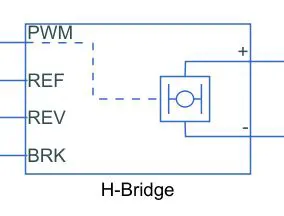
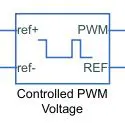
• This block represents an H-bridge motor drive. The block can be driven by the Controlled PWM Voltage block in PWM or Averaged mode.
• In PWM mode, the motor is powered if the PWM port voltage is above the enabled threshold voltage.
• In Averaged mode, the PWM port voltage divided by the PWM signal amplitude parameter defines the ratio of the on-time to the PWM period. Connection REF is for the reference input. This combined with the PWM connected will form the pulse input for the H-Bridge. Here, the REF input is connected to the Electrical Reference (ground). Connection REV corresponds to the reverse motion of the motor which essentially means, the backward motion of the vehicle. Here, the backward motion of the vehicle is not accounted for and so, the port is connected to the electrical reference. Connection BRK is for the braking of the vehicle.
• Since, the PWM mode results in a huge amount of simulation time, Averaged mode is selected for this simulation. Load current characteristics are considered to be smoothed here.
  Also, regenerative braking is enabled for the simulation. This means, when the vehicle starts decelerating, the corresponding amount of charge will be feedback to the battery. Accordingly, the BRK input is connected.

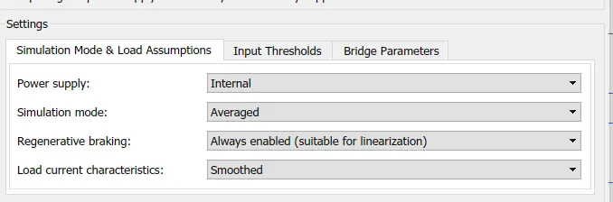
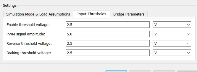
The Input Threshold parameters are left with their default values.

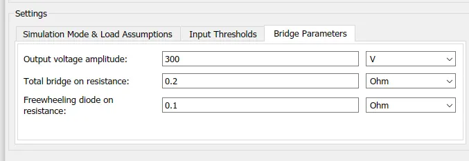
The Output Voltage Amplitude of the H-Bridge circuit is given the same value as the rated DC supply voltage of the DC motor.

Longitudinal Driver Block

A parametric longitudinal speed tracking controller for generating normalized acceleration and braking commands based on reference and feedback velocities.

Use the external actions to input signals that can disable, hold, or override the closed-loop commands determined by the block. The block uses this priority for the input commands: disable, hold, override.

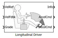
It is a parametric longitudinal speed tracking controller for generating normalized Acceleration and braking commands based on reference and feedback velocities.
The VelRef port is the reference velocity port where the input drive cycle data is fed.
The VelFdbk port corresponds to the feedback velocity. The actual velocity output given by the vehicle body is connected here. By comparing the actual(feedback) velocity with the reference velocity, the driver block generates acceleration and braking signals in order to minimise the error between the two concerned velocities. Grade corresponds to the grade angle. For this simulation, no inclination is considered and hence, a constant block with value 0 is connected. Info gives the output for the bus signal for different block calculations like the difference in reference vehicle speed and vehicle speed, etc. AccelCmd & DecelCmd correspond to the acceleration and deceleration commands generated respectively and are connected to the correspondingports of the Controlled PWM Voltage block.
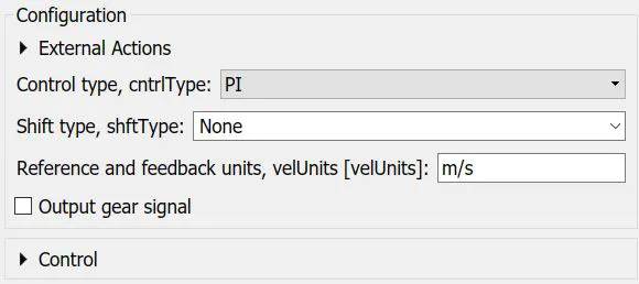
Here, the selected control type is PI Accordingly, the block implements proportional-integral (PI) control with tracking windup and feed-forward gains.

Battery Pack

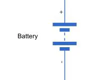
To model the Battery pack, a simple Battery block is used. This is because, if the generic battery block is used instead, the simulation will run for a much longer time.
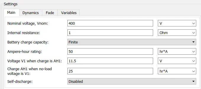
Here, the selected option for Battery Charge Capacity is Finite Accordingly, the block models the battery as a series internal resistance plus a charge-dependent voltage source. If the chosen option had been Infinite, the voltage source would have been constant. Also, the self-discharging of the battery and the battery dynamics is disabled.
The Battery Nominal Voltage is given as 400V
The Ampere-hour rating is assumed to be 50
The rest of all parameters are left with their default values.

Reference Drive Cycle

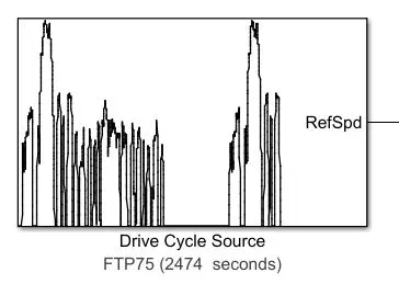
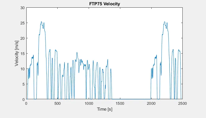
Here the selected Drive cycle is FTP75 and the plot of the drive cycle is shown below

Final Model

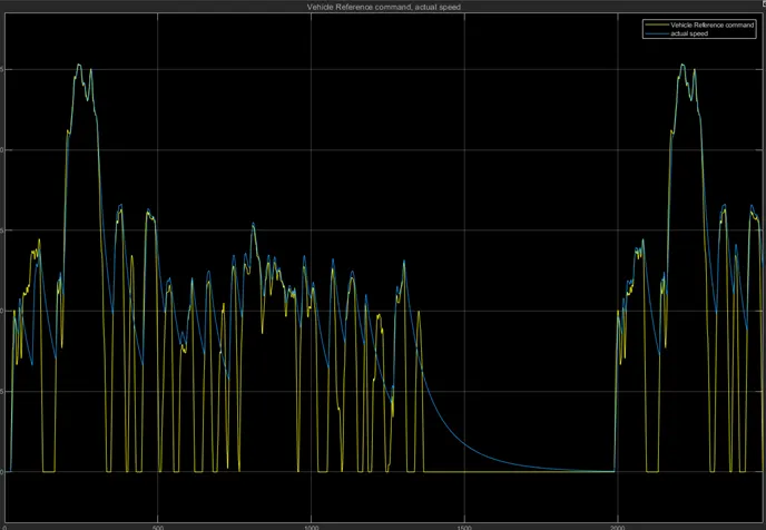
Results for the above model

• For the above model, the simulation time is taken for 2474 and the output plots are shown below

ref speed vs Actual speed

As can be seen from the above picture, the actual velocity of the vehicle differs from the reference drive cycle velocity. This is because the chosen battery capacity and motors are not able to propel the speed up to the required extent. If a battery of higher capacity is chosen, the actual velocity will tend to match with the reference velocity. Also, it may be noted that in certain regions, despite the drive cycle showing small decelerations, the vehicle actually

the Current consumed while the distance covered is shown below

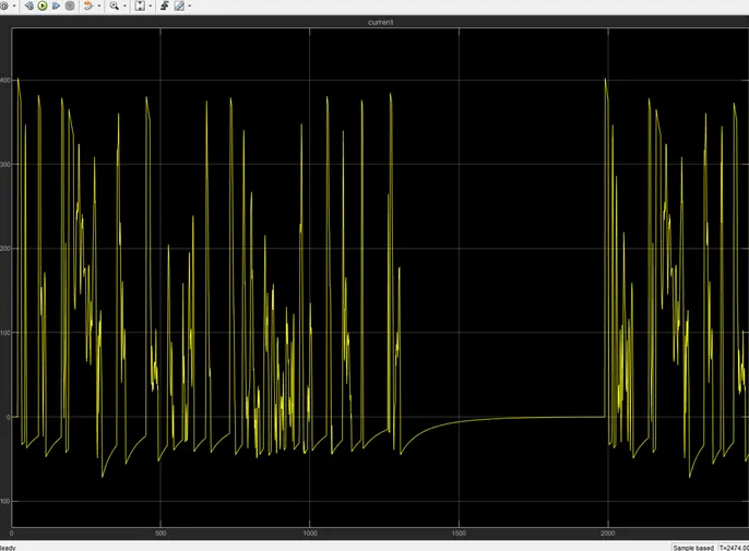
This means that the battery is not completely drained at the end and the vehicle can run on the same drive cycle a few more times before the battery soc becomes 0. Also, the thing to be noted here is, since we had enabled the regenerative braking for the simulation, the battery SOC increases slightly whenever the vehicle undergoes heavy deceleration. Again, this depends upon the generating tendency of the motor and the maximum amount of current that the battery can take.

CONCLUSION

• The model was successfully run for simulation under the standard FTP75 drive cycle. The results have been properly analyzed. Also, learnt quite a lot of interesting things like
• how to model an EV and carry out a real-time simulation
• how a motor controller works and what role it plays in the control of the electric motor
• how to calculate the SOC of the battery different powertrain blocks provided by Simulink which can be used to simulate a vehicle mode