Final Project: Design of an Electric Vehicle

Matlab Modelling Of Electrical car

Aim:

To create a matlab model of an Electrical car and to analyze and create a report about it.

Purpose:

Because of the depletion of fossil fuels and pollutions caused by burning the fuels affects the environment. And additionally day by the cost of the fuel also increases. This paves the way to the entry of electrical vehicles which uses the electrical energy, the cleanest energy. It does not produce any pollution. Yeah technology is growing day by day may be in future there will be another equivalent form of energy such as HYDROGEN which is as clean as electrical energy. Now let us discuss about the present, electrical vehicle.

Software used:

• Matlab/ Simulink

Main Components in Electric car:

• Battery
• Power Controller
• Motor
• Vehicle Body

Simulink Model:

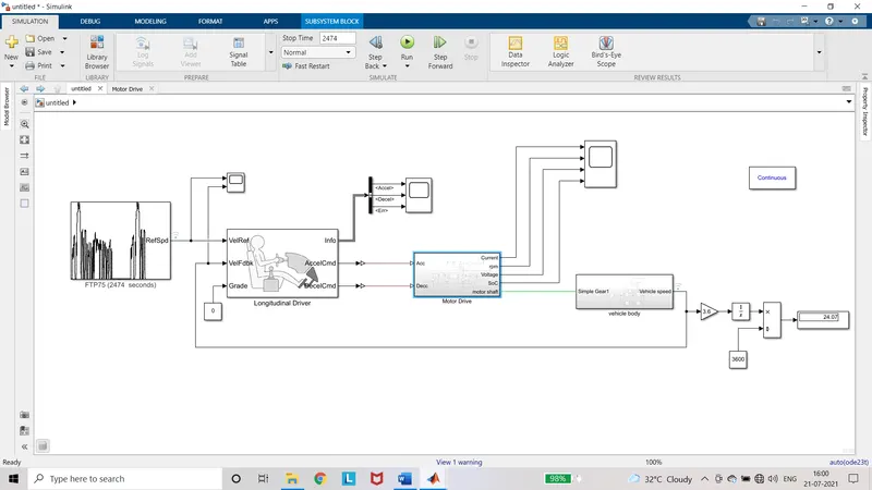
Blocks Used:

• Drive cycle source
• Longitudinal driver
• Controlled Voltage Source
• Controlled PWM Voltage
• H- Bridge
• Current sensor
• Voltage Sensor
• Brushed DC motor
• Mechanical rotational sensor
• PS terminator
• Battery
• Controlled current source
• Electrical reference
• Mechanical rotational reference
• Solver Configuration
• Discrete time integrator
• Gain
• Constant
• Rate transition
• Simple Gear
• Tire (Magic formula)
• Vehicle Body
• PS constant
• PS-Simulink converter
• Simulink-PS converter
• Sum
• Integrator
• Divide
• Display
• Powergui

Explanation and Configuration of Components used:

For better understanding let us go from backward.

Vehicle Body:

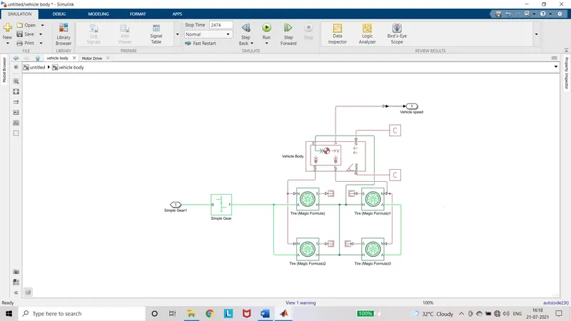
Vehicle Body block:

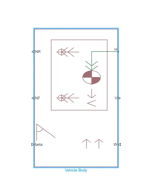
This block represents a two-axle vehicle body in longitudinal motion. The block accounts for body mass, aerodynamic drag, road incline, and weight distribution between axles due to acceleration and road profile. We can also include pitch and suspension dynamics or additional variable mass and inertia. The vehicle does not move vertically relative to the ground.

Connection H is the mechanical translational conserving port associated with the horizontal motion of the vehicle body. Connections V, NF, and NR are physical signal output ports for vehicle velocity and front and rear normal wheel forces, respectively. Connections W and beta are physical signal input ports corresponding to headwind speed and road inclination angle, respectively. M represents the additional mass.

Configuration:

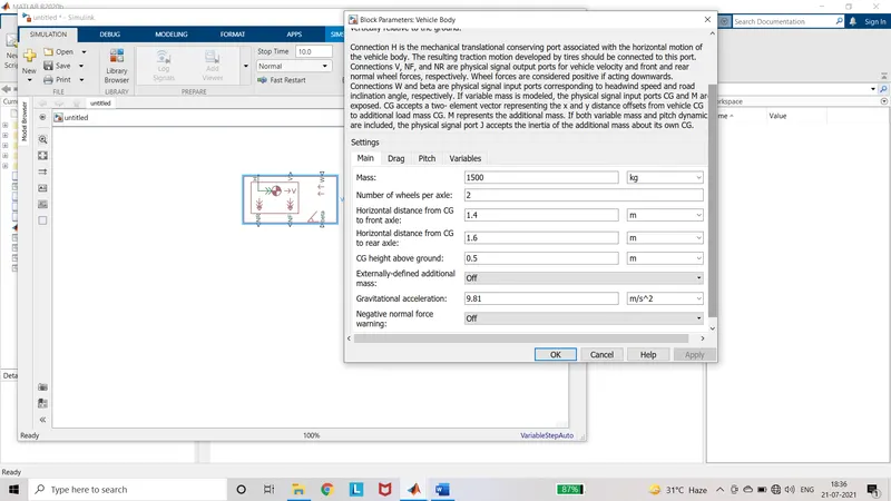
The mass is set to 1500kg.

Tire (Magic formula):

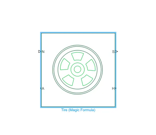
This block represents the longitudinal behaviour of a highway tire characterized by the tire Magic formula. The effects of tire inertia, stiffness, and damping can be included.

Connection A is the mechanical rotational conserving port for the wheel axle. The rotational output from the Simple gear is given to this port. Connection H is the mechanical translational conserving port for the wheel hub through which the thrust developed by the tire is applied to the vehicle. The H port from the vehicle body is connected to this port. Connection N is a physical signal input port that applies the normal force acting on the tire. The NR and NF from the vehicle body is given to this port accordingly. Connection S is a physical signal output port that reports the tire slip.

The parameters are kept default and rolling resistance is neglected.

Simple Gear:

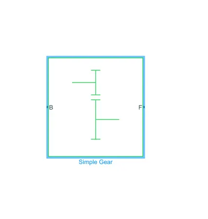
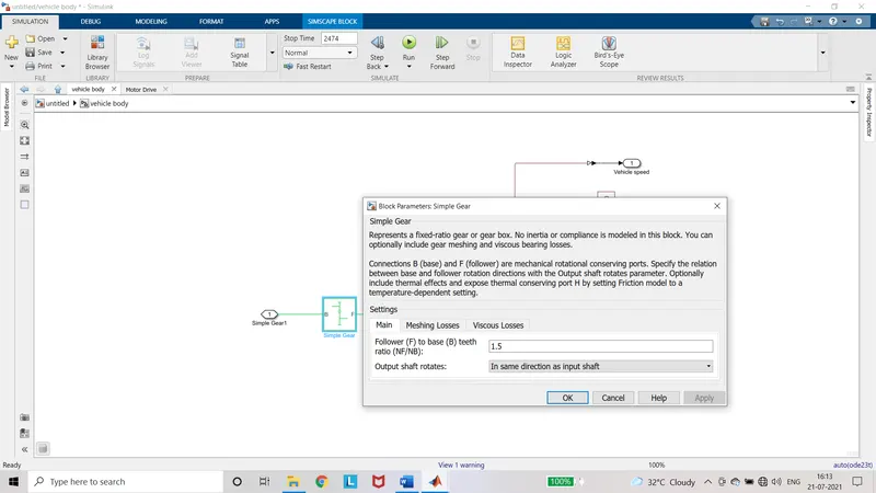
This block represents a fixed-ratio gear or gear box. The gear meshing and viscous bearing losses can be included if needed.

Connections B and F are base and follower which are mechanical rotational conserving ports. It specifies the relation between base and follower rotation directions with the Output shaft rotates parameter.

Configuration:

The value of gear ratio is changed to 1.5 and direction of rotation of output shaft set as same as input shaft.

Motor Drive:

Controlled voltage source:

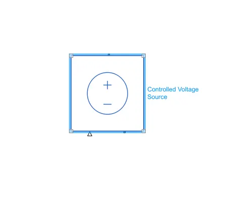
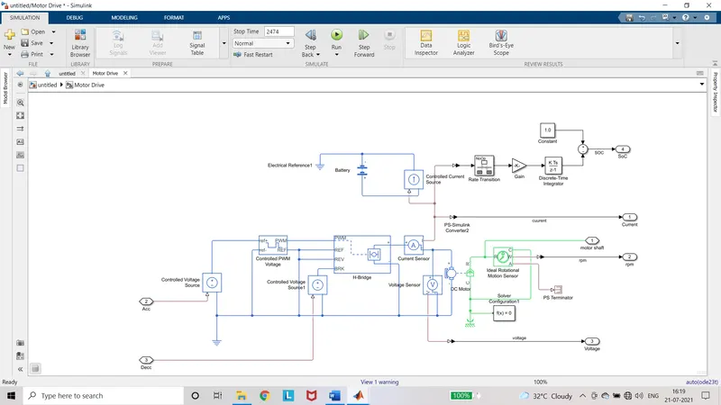
The block represents an ideal voltage source that is powerful enough to maintain the specified voltage at its output regardless of the current passing through it. The output voltage is V = Vs, where Vs is the numerical value presented at the physical signal port.

The input to the physical signal port is given from the Accelerator command of the Longitudinal driver.

Controlled PWM voltage:

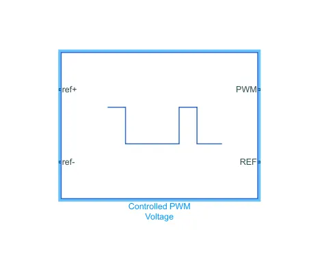
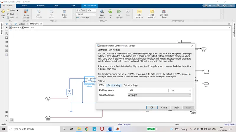
This block creates a Pulse-Width Modulated (PWM) voltage across the PWM and REF ports. The output voltage is zero when the pulse is low, and is equal to the Output voltage amplitude parameter when high. Duty cycle is set by the input value. The voltage from the controlled voltage source is given to the ref+ port. The ref- port is connected to the ground.

The Simulation mode can be set to PWM or Averaged. In PWM mode, the output is a PWM signal. In Averaged mode, the output is constant with value equal to the averaged PWM signal.

Configuration:

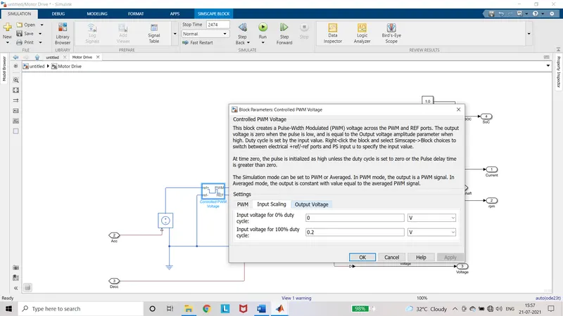
The simulation mode is set to averaged for the faster simulation. The output voltage at 100% duty cycle is set to 0.2V. Other parameter are set to default.

H – Bridge:

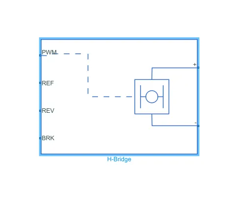
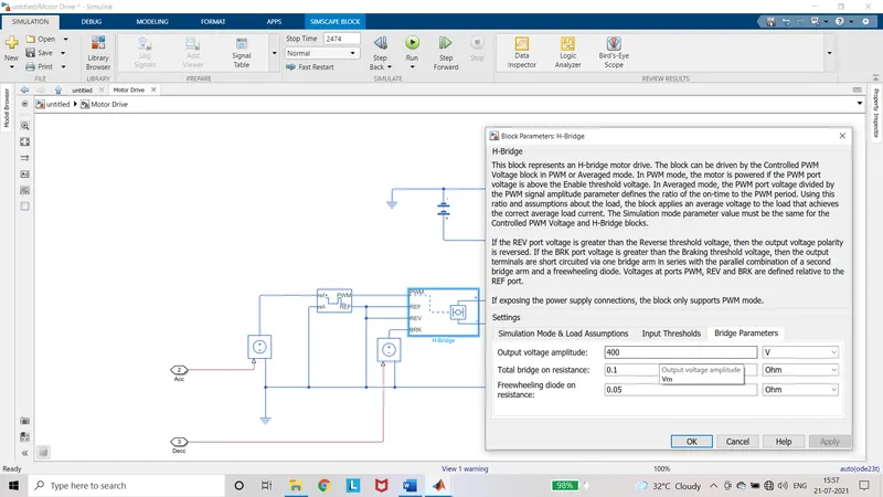
This block represents an H-bridge motor drive. The block can be driven by the Controlled PWM Voltage block in PWM or Averaged mode. In PWM mode, the motor is powered if the PWM port voltage is above the Enable threshold voltage. In Averaged mode, the PWM port voltage divided by the PWM signal amplitude parameter defines the ratio of the on-time to the PWM period. Using this ratio and assumptions about the load, the block applies an average voltage to the load that achieves the correct average load current. The Simulation mode parameter value must be the same for the Controlled PWM Voltage and H-Bridge blocks.

If the REV port voltage is greater than the Reverse threshold voltage, then the output voltage polarity is reversed. If the BRK port voltage is greater than the Braking threshold voltage, then the output terminals are short circuited via one bridge arm in series with the parallel combination of a second bridge arm and a freewheeling diode. Voltages at ports PWM, REV and BRK are defined relative to the REF port. The PWM port and REF port is connected to the PWM output port and REF output port of controlled PWM voltage. The REF and REV ports are connected to the ground. The BRK port is connected to the controlled Voltage source which is controlled by the Deceleration command from the Longitudinal Driver.

Configuration:

The simulation mode is set to averaged. The regenerative braking is set to always enabled. Output voltage amplitude is set to 400V which is given to brushed DC motor. Other parameters of the blocks are set to default.

DC motor:

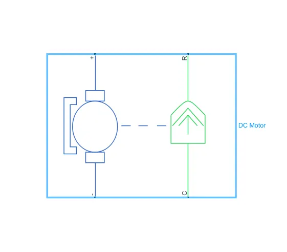
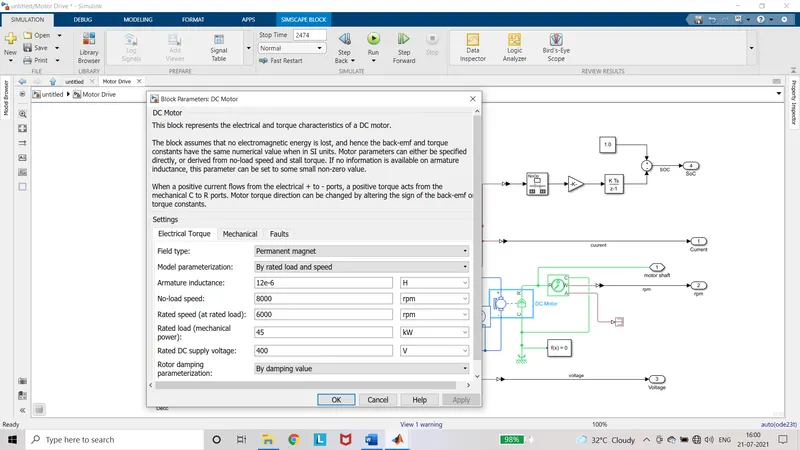
This block represents the electrical and torque characteristics of a DC motor. It assumes that no electromagnetic energy is lost, and hence the back-emf and torque constants have the same numerical value when in SI units.

When a positive current flows from the electrical + to - ports, a positive torque acts from the mechanical C to R ports. Motor torque direction can be changed by altering the sign of the back-emf or torque constants. The input to the motor is given by the H-Bridge. The port C is connected to ground and the port R is the mechanical rotational port connected to the simple gear.

Configuration:

The model parameterization is set to by rated load and speed. The no load speed and rated speed is set to 8000 rpm and 6000 rpm. The rated load is set to 45KW. And Rated Dc supply voltage is set to 400V. All other values are set to default.

Current Sensor and Voltage Sensor:

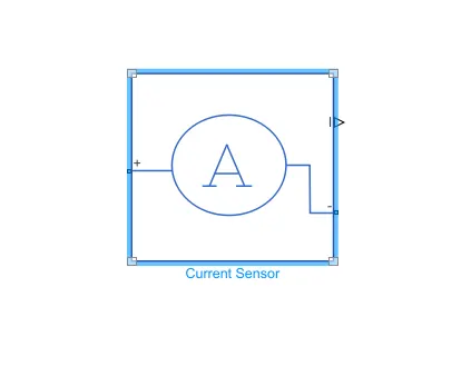
The ideal current sensor is a device that converts current measured in any electrical branch into a physical signal proportional to the current. It is used to measure the current to motor.

Connections + and - are conserving electrical ports through which the sensor is inserted into the circuit. Connection I is a physical signal port that outputs current value.

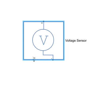
The ideal voltage sensor is a device that converts voltage measured between any electrical connections into a physical signal proportional to the voltage. It is used to measure the voltage applied to motor.

Connections + and - are conserving electrical ports through which the sensor is connected to the circuit. Connection V is a physical signal port that outputs voltage value.

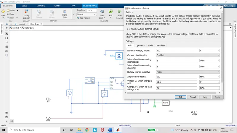
Controlled Current Source and Battery:

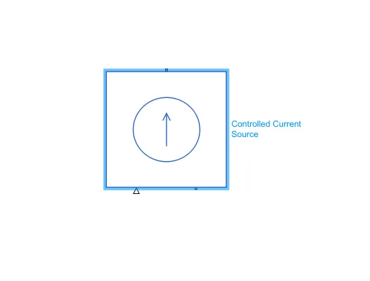
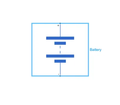
An ideal current source is powerful enough to maintain the specified current through it regardless of the voltage across it. The output current is I = Is, where Is is the numerical value presented at the physical signal port. This physical signal port is connected to the physical signal port of the current sensor. The positive this block is connected to the negative of battery and negative port to positive of the battery for the charging of battery.

The battery is used to deliver and store the energy.

Configuration:

The nominal voltage is set to 600V and current directionality is enabled. Battery charge capacity is set to finite and the Ampere hour rating is set to 150hr*A. All other parameters are set to default.

Gain for SoC:

Configuration:

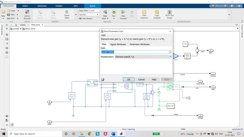
The gain value is set to 1/(AH*3600). The value for variable AH is set as 150.

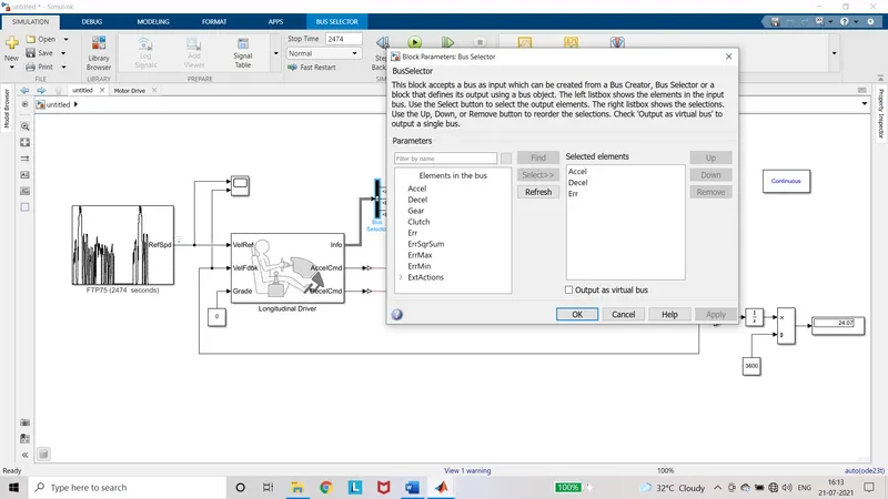
Longitudinal Driver:

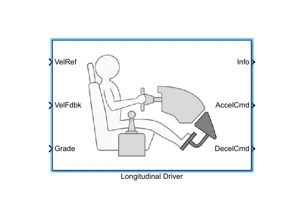
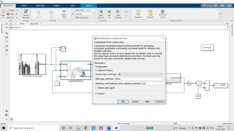
A parametric longitudinal speed tracking controller for generating normalized acceleration and braking commands based on reference and feedback velocities.

Use the external actions to input signals that can disable, hold, or override the closed-loop commands determined by the block. The block uses this priority for the input commands: disable, hold, override. The VelRef is connected to the output of the Drive cycle source. The VelFdbk is connected to output port V of the vehicle body.

Configuration:

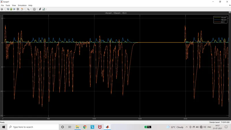
The grade is connected to the constant and is set to zero. AccelCmd and DecelCmd are connected to motor drive. Info is connected to Bus selector from which Accel, Decel and Err is selected and connected to scope.

Drive Cycle Source:

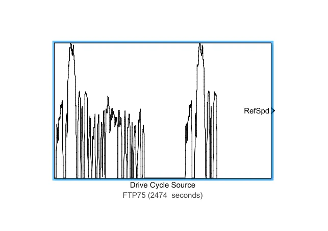
Drive cycle source generates a standard or user-specified longitudinal drive cycle. The block output is the vehicle longitudinal speed. You can import drive cycles from:

• Predefined sources such as FTP75, WOT, US06, etc
• Workspace variables, including arrays and time series objects
• mat, xls, xlsx, or txt files

Configurations:

The drive cycle source is set to FTP75. Update the simulation time.

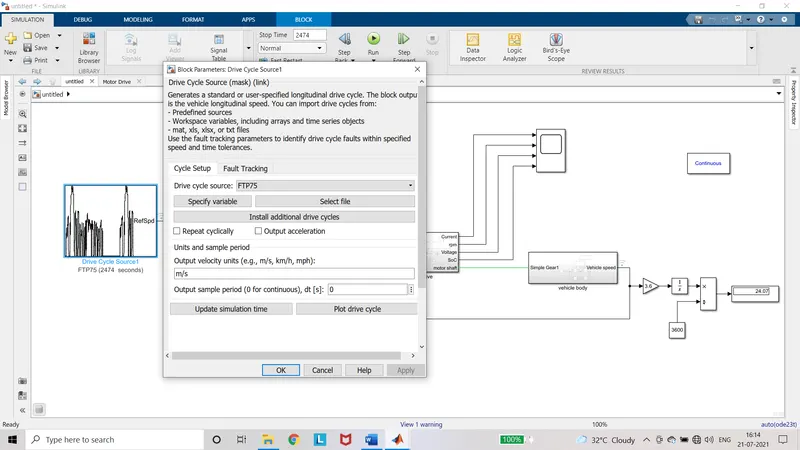
And finally the velocity from the vehicle body is converted from m/s to kmph by adding the gain block. It is then integrated and divided by 3600 to get the distance in kmph. This is displayed in the display.

The simulation is run with the above parameterization values and output is visualized in the scope.

Output:

Scope for Accel, Decel, Err commands:

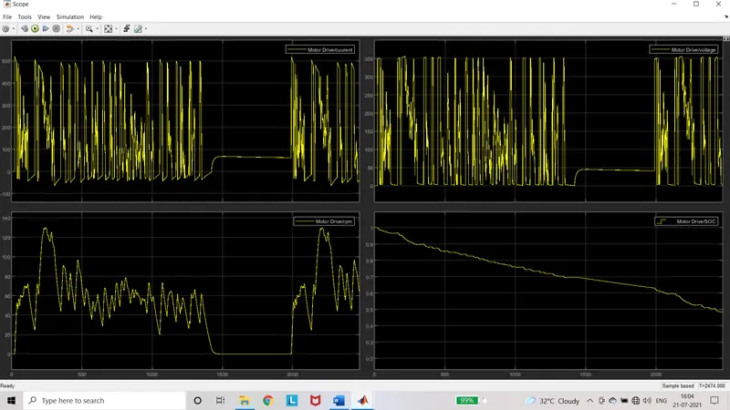
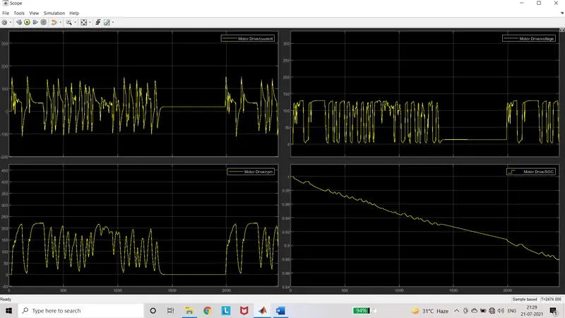
Scope for Motor Current, Voltage, Speed and State of Charge (SoC):

Analysis:

When the acceleration command is given according to the level of acceleration the voltage and current is given to the dc motor and speed is varied accordingly. When the deceleration or brake command is given the voltage is zero and current is negative to motor and the speed is zero gradually but not suddenly due to the weight of rotor. The negative current means the regenerative braking happens and charge the battery. The state of charge is reduced during the acceleration command. If the acceleration command is suddenly increased the state of charge also reduces to some great extent. During the deceleration or brake command the state of charge reduces slowly due to the power required to stop. During this period the regenerative braking is also involved for small amount of time.

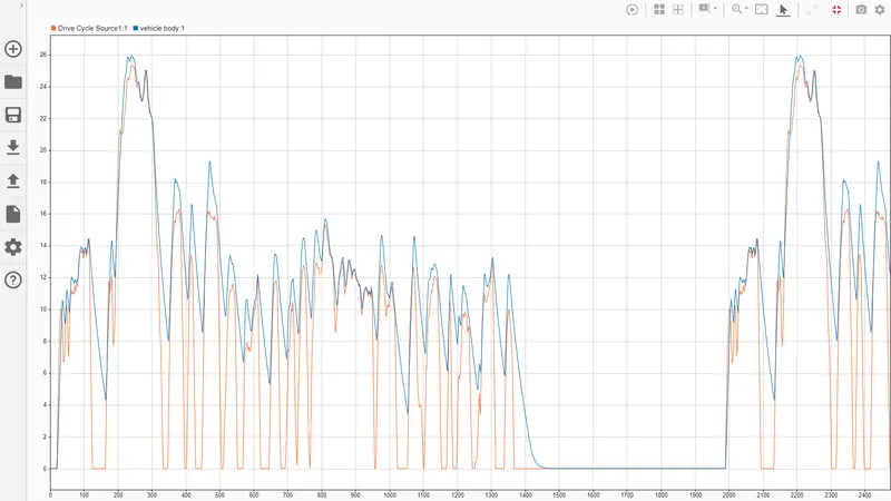
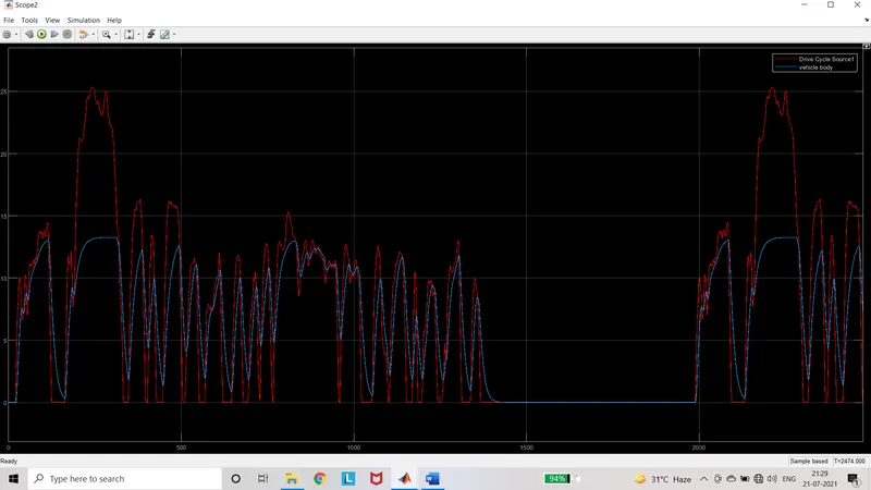
Scope for Drive cycle and Vehicle Velocity:

Analysis:

The velocity of both reference drive cycle and the vehicle body is visualized. When the reference drive cycle is reduced to zero, the vehicle body does not come to zero immediately. The speed will gradually decreases and then come to zero.

The distance covered by the vehicle is 24.07km with the remaining SoC of 48%.

Case study:

By changing Gear ratio:

If the gear ratio is increased to 5 from 1.5 then the drive cycle reference speed and Vehicle body speed is more or less same. The error is very less.

The state of charge also is more at the end of the simulation.

The distance covered by the vehicle is 19.83km with the remaining SoC of 86%.

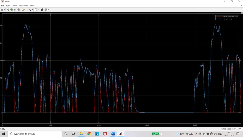
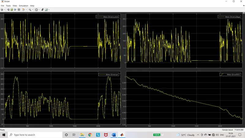
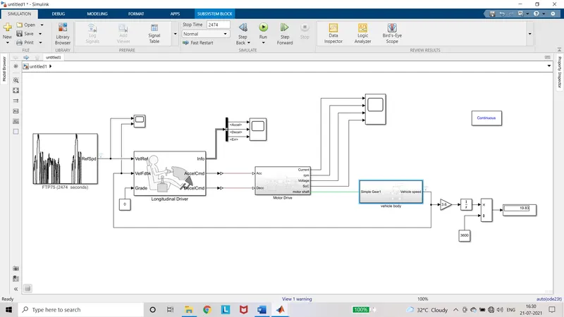
The Speed of vehicle is operated near the desired drive cycle reference. Whenever the brake is applied or deceleration command is given the current is negative due to the generating action of the motor. The regenerative braking is efficient and it charge the battery. This was clearly seen in the above scope.

By changing the input value of 100% duty cycle in controlled PWM voltage:

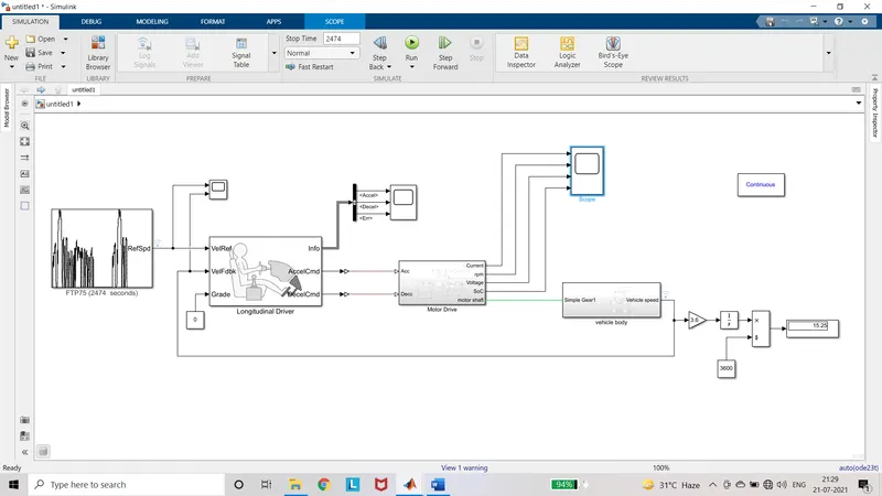
When the input value of 100% duty cycle in controlled PWM voltage is changed the velocity of vehicle also changes. When the input value of 100% duty cycle is increased from 0.2 to 3, the speed of vehicle body decreases. The distance travelled also decreased to 15.25km. The state of charge at the end of drive cycle is 88%.

Result:

The vehicle speed and the SoC of the battery is varied by changing the gear ratio, input voltage at 100% duty cycle of controlled PWM voltage and the capacity of the battery excluding the wind velocity and grade. So by changing these parameters and by calculating the efficiency, among that for which value the maximum efficiency obtained is considered for modelling the Electrical car.

All the images and the matlab model file are uploaded in the drive and drive link is shared.

Drive Link:

https://drive.google.com/drive/folders/1X1bD5LiblFgfqzf1x3Gi9H5rFL6pXuwa?usp=sharing