Final Project: Design of an Electric Vehicle

Create a MATLAB model of an electric car which uses a battery and a DC motor. Choose suitable blocks from Powertrain block set. Prepare a report about your model including following:

Objectives:

1. System level configurations

2. Model parameters

3. Results

4. Conclusion

Block Diagram of an EV:

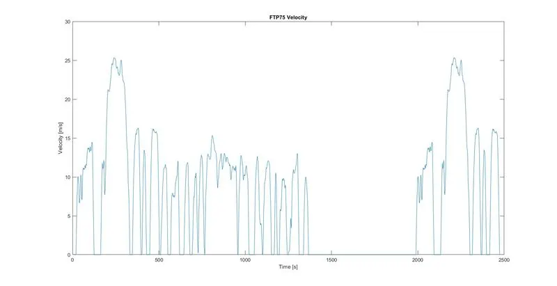
In the designed EV main blocks are Battery, drive cycle, motor, motor controller, vehicle body, and transmission system. Drive cycle is the input data like how a human drives his actual vehicle here FTP75 drive cycle is introduced to make the designed vehicle to give the output how it reacts to the drive cycle. The main object to design the EV is to obtain the speed by the driver, to estimate the state of charge (SoC), distance traveled by the vehicle. There is a soc block that will estimate the state of charge of the battery, distance is calculated by the speed and time parameters.

1. Vehicle Body Block:

This is the first block to start modeling an EV. This block consists of a vehicle chassis, tires, and gearbox, a simple type of gear. This means the block contains the properties like normal forces, mass, velocity, etc.

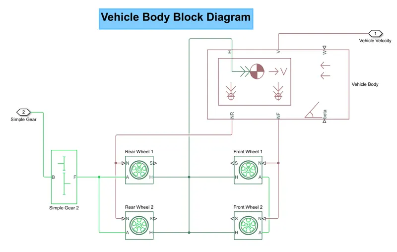
• Tire Block:

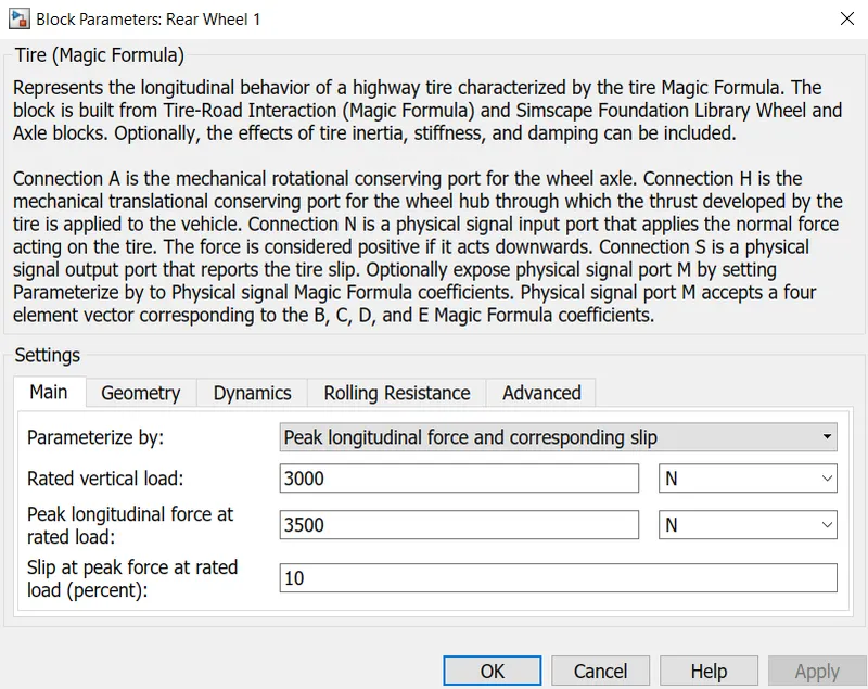
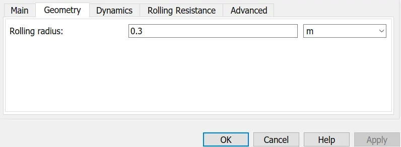
The tire block used is a multifunction type where it has 4 inputs. These are as follows

1. A - Axles
2. S - Slip
3. H - Hub
4. N - Normal Force

These are then connected to the vehicle body.

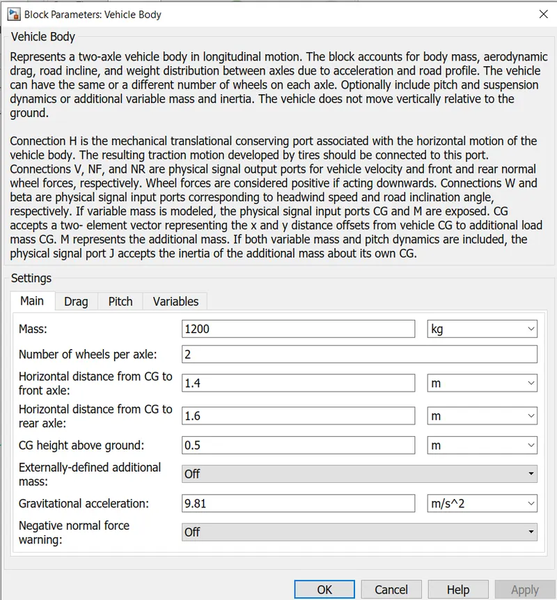
• Vehicle Block:

The vehicle body has various inputs that can be modeled for the vehicle to have a basic setup. It consists of 3 input and 3 output ports. Which are as follows

Inputs

1. W - Headwind speed
2. Beta - Inclination angle
3. H - Hub Connection

Outputs

1. V - Longitudinal Velocity
2. NF - Front axle normal force
3. NR - Rear axle normal force

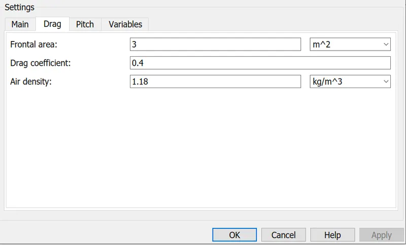
In this model, I took wind velocity and inclination as zero.

• Simple Gear Block:

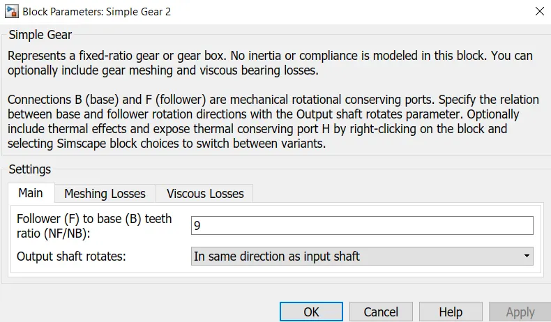
In the vehicle body model, we have connected a simple gear system to transmit the power from the motor to the wheels. The gear ratio has been changed to 9 and the 'the output shaft is rotating in the same direction as the input' option is activated.

fig of Simple gear

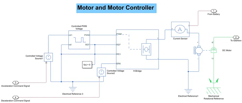
2.Motor and Motor controller (PWM):

• Motor Block:

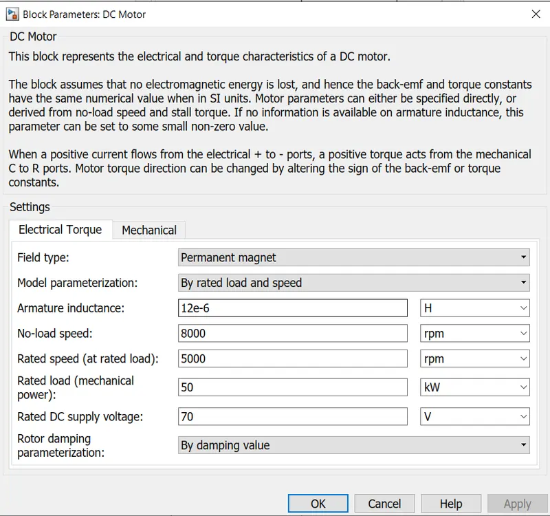
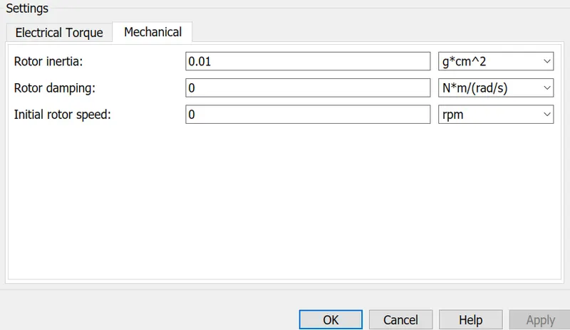
For this model, I have used a simple brushed DC Motor. There are certain parameters that are very important to choose a certain type of motor like armature inductance, rated power, rated torque, etc.

The inductance of armature is the reason why the power of a motor can be smaller than the product of RMS voltage and RMS current, and a power factor needs to be applied.

This basically means that the armature inductance governs the amount of power required by the motor to be delivered to the wheels. This power may be very small so as to move a vehicle or very high as to move the vehicle at top speed. Basically, the armature is the moving part of the motor that produces the emf which turns to power the motor.

Torque constant is basically the torque a motor is limited to produce in an hour.

• H-Bridge Block:

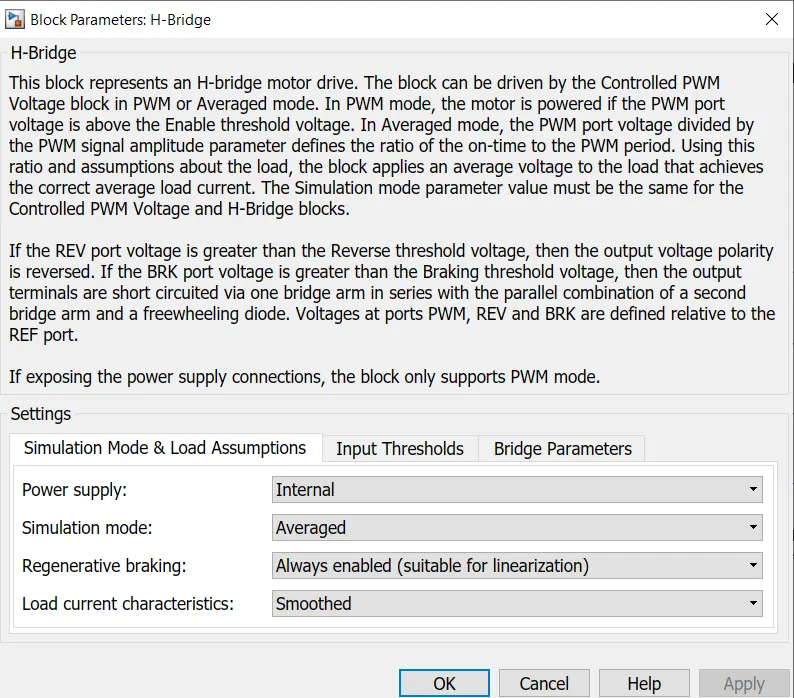
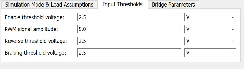
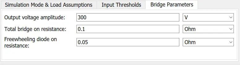
The H-Bridge block represents an H-Bridge motor driver. As we want to linearized our model we used the averaged mode and the operating point is set as shown below.

This block includes six ports, which are given below

• + - Positive load connection port
• - - Negative load connection poet
• PWM - Pulse-width modulated signal
• REF - Reference
• REV - Reverse case signal
• BRK - Brake case signal

• Controlled PWM Voltage Block:

For any motor to run we need a controller to control the voltage and current supply from the battery . For this model I have used a PWM averaged model that takes the input from the duty cycle and feedback from a longitudinal driver.

This averaged block also consists of ports for connections of the battery pack and motor. This block calculates the duty cycle based on the reference voltage across ref+ and ref- ports. There are four ports such as

• ref+ - Positive terminal
• ref- - Negative terminal
• PWM - Pulse-width modulated signal
• REF - Floating zero volt reference

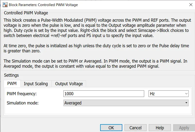
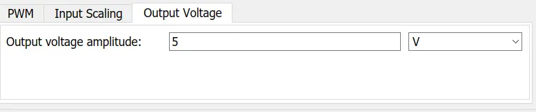
The modeling is done only for forward motoring and regenerative braking. So to accomplish this we have to feedback the voltage generated during braking to the battery, it is done using two controlled voltage sources in order to make both possibilities.

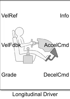
3. Longitudinal Driver:

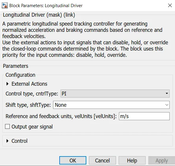
This model consists of the commands that a driver will give the vehicle and based on those commands the various scopes are added to monitor the output from the driver. This block is called a longitudinal driver.

This block takes various parameters as a reference to the vehicle like velfdbk and velref.

VelRef takes the input from the drive cycle that we use for the simulation. For this simulation of EV, we have used the FTP75 cycle.

4. Battery and Battery Management System:

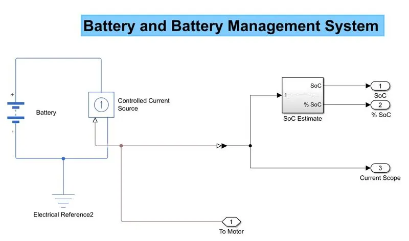
• SoC Estimate:

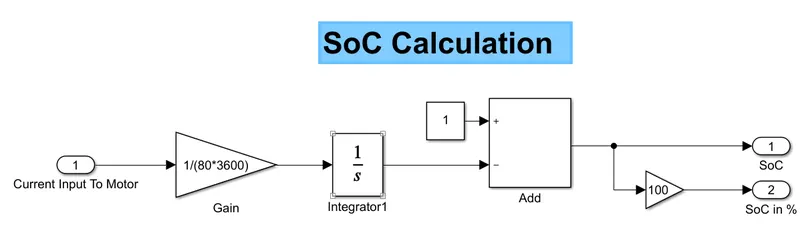
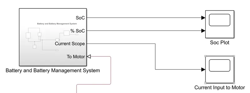
By connecting the battery directly to the motor we lose the control aspect of the motor so we use a controlled environment to model a battery-like simulation so we can simulate the current and state of charge (SoC). Here one end of the battery connected to the ground and the other one is connected to the motor through a current sensor so that we can measure the current input to the motor. By using this current integrating and dividing by (mAh*3600) we get the charge dissipated and comparing it with 1 or 100% we can get the SoC of the battery.

RESULTS:

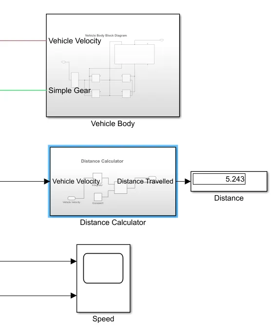
• For the results, we have attached much output capturing scopes in the model. For these outputs, we need to make sure that we have the proper connections. We have used a normal body subsystem that has two outputs connecting to the motor and to a feedback scope.

• In the above figure, we can see that the body is connected to the motor via the rotor output. This R output is connected to the simple gear we have used in the body subsystem. The cage is connected to a mechanical reference so as to show the stationary nature of the motor. The speed connection of the motor is then connected to scope and to an integrator and a divider block that gives us the distance output that the vehicle will run for the given drive cycle.

SoC Analysis:

• For the state of charge, we can observe some dips and some constant regions. These dips are mainly observed on acceleration feedback from the longitudinal driver to the PWM averaged block and to the battery. The constant regions in the SoC graph are the areas where the battery is in regenerative braking or in the deceleration feedback mode. The ups in the graph are due to the charging of the battery.

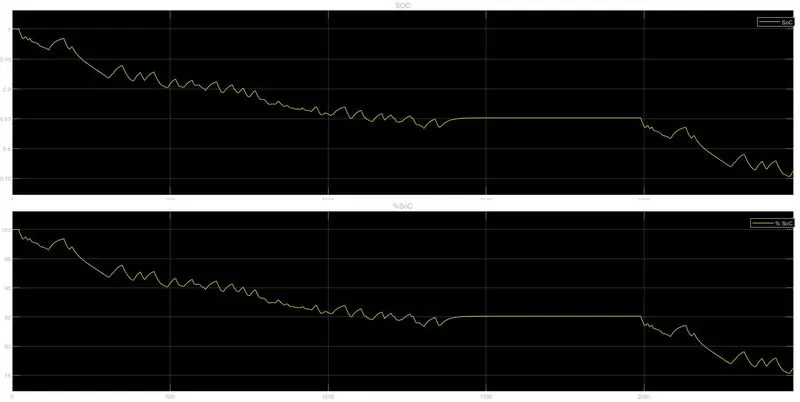
• Regenerative braking is an energy recovery mechanism that slows down a moving vehicle or object by converting its kinetic energy into a form that can be either used immediately or stored until needed. In this mechanism, the electric traction motor used the vehicle's momentum to recover energy that would otherwise be lost to the brake discs as heat. This contrasts with conventional braking systems, where the excess kinetic energy is converted to unwanted and wasted heat due to friction in the brakes, where the energy is recovered by using electric motors as generators but is immediately dissipated as heat is resistors. In addition to improving the overall efficiency of the vehicle, regeneration can significantly extend the life of the braking system as the mechanical parts will not wear out very quickly.

• From the battery block we can also observe the current profile for the FTP75 cycle.

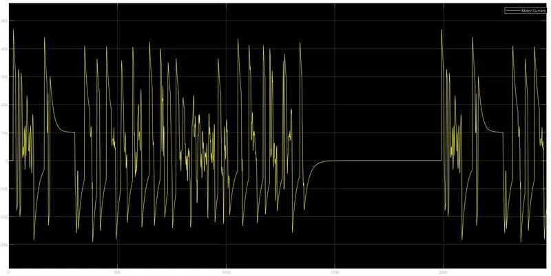
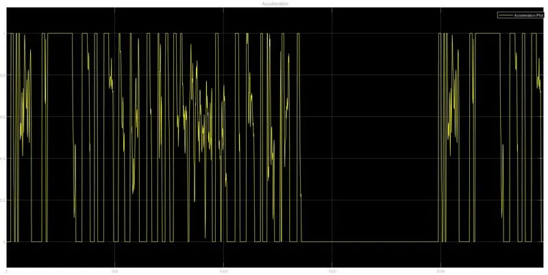
• When we talk about the acceleration and deceleration of the graph cycle we know that the vehicle has accelerated or decelerated at many time stamps. Basically, the driver has pressed the accelerator and decelerator many times during the drive cycle. Maybe he was in a traffic situation where he needed to brake and move forward on simultaneous occasions.

• For the main output, we have put a scope with two inputs. One input is the vehicle feedback and the other is the speed of the vehicle. For our simulation of the vehicle to run perfectly, we need a match on the drive cycle for the position and the speed.
• The maximum speed the drive cycle can attain is 20 kmph.

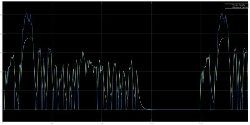
• From the graph, we can see that the drive cycle is almost identical to the speed output we get from the simulation.

CONCLUSION:

The modeled EV has obtained an output according to the FTP75 drive cycle and it can be tested for any drive cycle by selecting in the drive cycle block. It has traveled 5.24 km by the present 80 Ah battery capacity if we increase the battery capacity to higher levels we can travel more distance but in real time this should be done by considering the space and cost.