FINAL INDEPENDENT PROJECT

AIM

To write a code for mathematical analysis of Two Bar Mechanism and Four Bar Mechanism.

OBJECTIVES

• Mathematical analysis , Velocity Analysis for two bar mechanism .
• Plotting graph for Variation of link  theta 1 and theta 2 and Variation of angular velocity  for two link.
• Mathematical analysis , Velocity Analysis ,  Acceleration analysis , Dynamic analysis  for four bar mechanism .
• Plotting graph for Polar load for each joint and Variation of Motor torque.

SCOPE OF PROJECT

A constrained rigid ody system in which one of the bodies is  in the frame is refered as mechanism . When considering rigid body system the degrees of freedom of that mechanism is important

For this project the analysis of a hypahical two bar mechanism which welds a structure in aproduction line carried out . The four bar mechanism would be driven by an electric motor was also analzed.

Four bar mechansim can be used for many  mechanical purposes convert rotational motion to recipracating motion (eg knee joint and suspension )

THEORY

2 BAR MECHANISM

A two bar linkage which is described  in differential equations can peform non linear behaviou due to system parameters or external input . As a basic component of robot system  the investigation  of its behaviour can improve robot perfomance , control stratergy and system parameters.

A two bar mechanism linkage as a basic component of mechanical system can perform nonlinear motions ,  among which chaotic motion is the most typically complicated one. It is known that the performance of such a mechanism is influenced by system parameters such as mass and friction coefficient , the intial states and external input such as  driving torque controlled by specially designed controler.

For a two bar linkages the motions of its two rotating links can be single periodic  , multiple periodic  , quasiperiodic and chatioc . 

VELOCITY ANALYSIS IN TWO BAR MECHANISM

To determine the velocity of different points on links of a mechanism for a given input motion . Determination of the motion characterstics of links in a mechanism is required for the force analysis .

Velocity of links and of points of mechanism can be determined by different methods 

• Relative velocity method or Velocity polygon method
• Instantaneous center method

                                                       

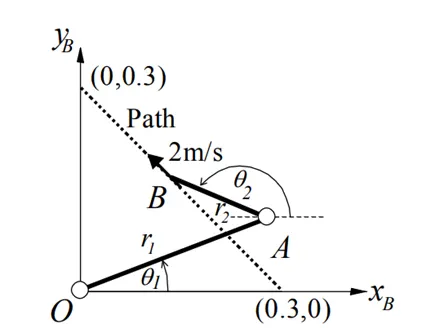
The two bar link  shown in figure consists of link OA which is fixated to the point of and the link AB at point A . To ensure that point B travels in straight line path in the XY coordinates from (0.3m, 0.0m) to (0.0m,0.3m) with a constant velocity of 2m/s  the angles theta 1 and  theta 2  will be controlled.

The inputs of the two bar link are following

r1=0.4m

r2=0.3m

where 

r1= Link OA length

r2= Link AB length

THE POSITION ANALYSIS 

For closed loop OABC :

Equation 1

 

Equation 2

Solving for both r1costheta and r1sintheta 1 gives:

Equation 3

Equation 4

By squaring and adding up both sides of the equations the mechanism position can be :

 Equation 5

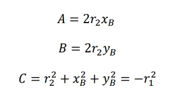
Now theta 2 is calculated

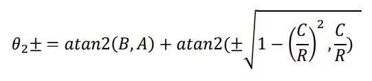
Equation 6

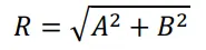
Equation 7

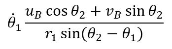
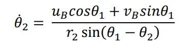
The angular velocity can be calculated using both Equation 1 and Equation 2 from above differentiating with respect to time

MATLAB CODE FOR TWO BAR

% SUBMITTED BY VIKAS
% FINAL INDEPENDENT PROJECT 
% MATHEMATICAL ANALYSIS,VELOCITY ANALYSIS  OF TWO BAR MECHANISM

 
clear all
close all
clc

% VARIABLE INPUTS
r1=0.4; 
r2=0.3; 
YB=sqrt(2); 
i=0; 
XB=-YB;

for X=0.3:-0.003:0;
    Y= -X+0.3; 
    A=2*r2*X; 
    B=2*r2*Y; 
    C=((r2)^2)+(X^2)+(Y^2)-((r1)^2);
    R=sqrt((A^2)+(B^2)); 
    Z=C/R; 
    zz=sqrt(1-(Z^2)); 
    i=i+1;

% POSITION ANALYSIS
TH2=atan2(B,A)+atan2(zz,Z);
if TH2<0; TH2=TH2+2*pi;end

TH2b=atan2(B,A)-atan2(zz,Z);
if TH2b<0; TH2b=TH2b+2*pi;end

TH1=atan2((Y-r2*sin (TH2)), (X-r2*cos (TH2)));
T1(i)=TH1; T2(i)=TH2; T2b(i)=TH2b;


% VELOCITY ANALYSIS
w1=((XB*cos (TH2)) + (YB*sin (TH2)))/(r1*sin (TH2-TH1)); 
w2=((XB*cos (TH1)) + (YB*sin (TH1)))/(r2*sin (TH1-TH2)); 
W1 (i)=w1; 
W2 (i)=w2;

end

% PLOTTING

figure (1) 
plot (T1*180/pi,'LineWidth',3,'Color','g'); 
hold on 
plot (T2*180/pi,'LineWidth',3,'Color','y'); 
grid; 
title('VARIATION OF LINKS')
xlabel('y_B (m)') 
ylabel('\Theta (degree)'); 
legend('\Theta_1','\Theta_2'); 
xlim ( [0 100]) 
ylim([-50 200]) 

% PLOT OF  ANGULAR VELOCITY FOR THEAT1 AND THETA 2
figure (2) 
plot (W1,'LineWidth',3,'Color','b'); 
hold on
plot (W2,'LineWidth',3,'Color','r'); 
grid 
title('VARIATION OF ANGULAR VELOCITY') 
xlabel('y_B (m)') 
ylabel('\omega (rad/sec)'); 
legend('\omega 1', '\omega 2');
xlim ( [0 100]) 
ylim([-3 14]) 

Variable inputs

clear all
close all
clc

% VARIABLE INPUTS
r1=0.4; 
r2=0.3; 
YB=sqrt(2); 
i=0; 
XB=-YB;

for X=0.3:-0.003:0;
    Y= -X+0.3; 
    A=2*r2*X; 
    B=2*r2*Y; 
    C=((r2)^2)+(X^2)+(Y^2)-((r1)^2);
    R=sqrt((A^2)+(B^2)); 
    Z=C/R; 
    zz=sqrt(1-(Z^2)); 
    i=i+1;

• clear all     Clear all the variables in workspace
• close all      Close all plots and figures
• clc              Clears the command window
• Defining the variable inputs for two bar
• For            loop is repetaion control structure  that allows you effeciently write a loop that needs to execute a specific number of times.
• i                imaginary unit

Position Analysis

% POSITION ANALYSIS
TH2=atan2(B,A)+atan2(zz,Z);
if TH2<0; TH2=TH2+2*pi;end

TH2b=atan2(B,A)-atan2(zz,Z);
if TH2b<0; TH2b=TH2b+2*pi;end

TH1=atan2((Y-r2*sin (TH2)), (X-r2*cos (TH2)));
T1(i)=TH1; T2(i)=TH2; T2b(i)=TH2b;

• Defining or inputing the equation 5 and 6

Velocity Analysis

% VELOCITY ANALYSIS
w1=((XB*cos (TH2)) + (YB*sin (TH2)))/(r1*sin (TH2-TH1)); 
w2=((XB*cos (TH1)) + (YB*sin (TH1)))/(r2*sin (TH1-TH2)); 
W1 (i)=w1; 
W2 (i)=w2;

• Inputing or defining the equation 7

Plotting

% PLOTTING

figure (1) 
plot (T1*180/pi,'LineWidth',3,'Color','g'); 
hold on 
plot (T2*180/pi,'LineWidth',3,'Color','y'); 
grid; 
title('VARIATION OF LINKS')
xlabel('y_B (m)') 
ylabel('\Theta (degree)'); 
legend('\Theta_1','\Theta_2'); 
xlim ( [0 100]) 
ylim([-50 200]) 

% PLOT OF  ANGULAR VELOCITY FOR THEAT1 AND THETA 2
figure (2) 
plot (W1,'LineWidth',3,'Color','b'); 
hold on
plot (W2,'LineWidth',3,'Color','r'); 
grid 
title('VARIATION OF ANGULAR VELOCITY') 
xlabel('y_B (m)') 
ylabel('\omega (rad/sec)'); 
legend('\omega 1', '\omega 2');
xlim ( [0 100]) 
ylim([-3 14]) 

• Plot        Creates the plot using specified line style, marker, color

RESULTS

                                                         

                        

                                                              

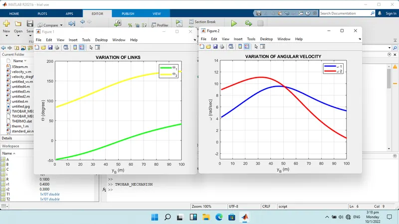
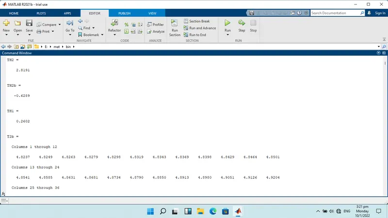
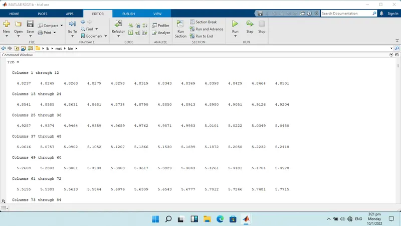
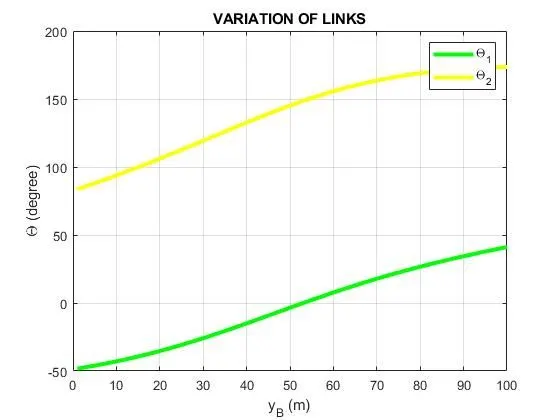
 Variation of link with angle theta1 and theta 2 . It is seen that both angles are positive as they rotate along the excesses in an anticlockwise direction . Theta 1 begins above 50 degree and increases to an angle of approxiamately 50 degree  indicating a continuous upward direction .Theta two on the other hand  starts in a positive position and begins to increase to points beyond 150 degrees easily

                                                                  

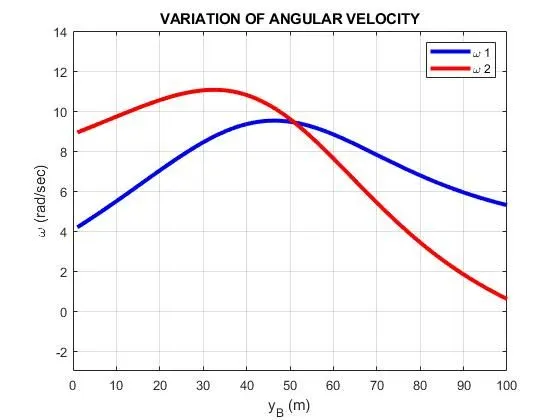
Variation of angular velocity . It is shown that the omega 1 begins a lower place than omega 2 , with omega 2 starting above 8 rad/sec /. An increase in velocity is noticed in the second angle when in comparsion to the first this is due to rapid acceleration . The first angular velocity has low peak point in the second angular velocity , but second angular velocity sees sharp decrease of this peak is reached when compared to first angular velocity.

FOUR BAR MECHANISM

                                                                           

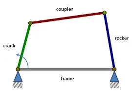
A four bar linkage also called as four bar is the simplest movable closed chain linkages . It consists of four bodies called bars or links connected in a loop by four joints . Generally joints are configured so that links move in parallel planes and assembly.

A four bar linkage is versatile mechanism that is widely used in machines to transmit motion or to provide mechanical advantage . Four bar linkages can also be used as function generators .  Thier low friction higher capacity to cary load ease of manufacturing and reliability of performance in spite of manufacturing tolerances make them preferable  over than other mechanism in certain applications . It is also the most fundamental linkage mechanism and many more complex mechanism contain  the four bar linkage as elements 

                                                       

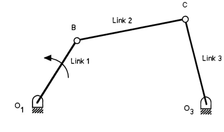
COMPONENTS OF FOUR BAR MECHANISM

 Link

Alink is one of the rigid bodies or members joined together . The term rigid link or sometimes simply  link is an idealization used in the study of mechanisms that does not consider small deflections due to strains in machine members.

Frame

The fixed or stationary link in a mechanism is called the frame . When there is no link that is actually fixed on elink may be considered as being fixed and determine the motion of the others  links relative to it.

Joint or Kinematic pair

The connections between links that permit relative motion are called joints . An unconstrained rigid body has a mobility of six degrees freedom . Each joint reduces the mobility of a system.

Lower Pairs and Higher Pairs

Connection between rigid bodies can be categorized as lower and higher pairs of elements . The two elements of a lower pair have a theortical surface contact with one another  while the two elements in the higher pair have theoratical points or line contact.

Kinematic Chain

A kinematic chain is an assembly of links and joints . In a closed kinematic chain link is connected to two or more other links.

Mechanism

A mechanism is a kinematic chain in which  one link is considered fixed for the purpose of analysis but motion is possible in other links.

Linkage

If kinemtic chain are needed to be examined without regard to its ultimate  use assemblage of rigid bodies connected by kinematics joints of lower pairs are identified as linkages

Motor torque 

The torque output of a motor is the amount of rotational force that the moptor develops .

 FOUR BAR MECHANISM

                                          

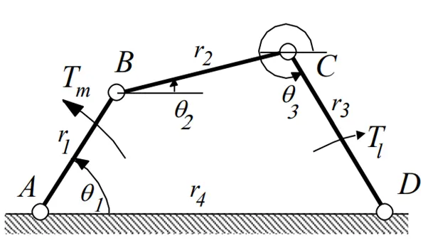
The four bar mechanism consists of three links link AB,BC,CD and DA  which represents the ground . Link AB is driven by a motor with torque force Tm starting the movement in the mechanism CD then carries the load torque TI . A counter clockwise direction is taken in  a horizontal axis to calculate the angles.

The Parameters given of the four bar mechanism as follows 

   LINK                      MASS (kg)                 LENGTH                  INERTIA (Kg.m2)            rG(mm)

    AB                            0.3                             10                            0.00002                              5

    BC                            0.5                             35                            0.005                                17.5

    CD                            0.6                             20                           0.00009                              15

    DA                            ---                             30                            --------                               ----

THE POSITION ANALYSIS

    

               

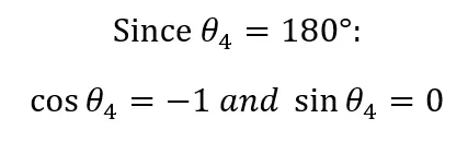
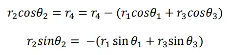
Giving the equations

By squaring and adding up both sides of equation the following equation are obtained

                      

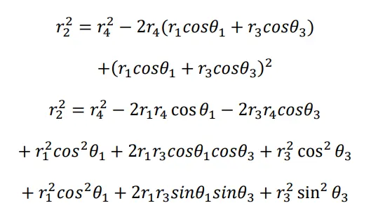
Therefore

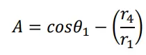
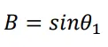
where 

         

           

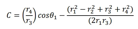
With solution to equation being

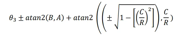
where

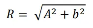
LINK POSITION

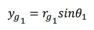
For MATLAB to be able to produce results the XY position of each link needs to be calculated .

Link AB

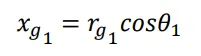
Link BC

Link CD

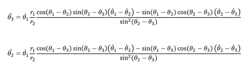
THE VELOCITY ANALYSIS

To calculate the angular acceleration the deriative of the equation above in the velocity analysis can be take 

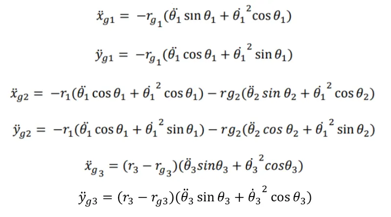
CENTER OF MASS ACCELERATION

The force condition on points A,B,C and D need tobe calculated to obtain the center of mass acceleration 

DYNAMIC ANALYSIS

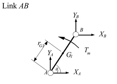
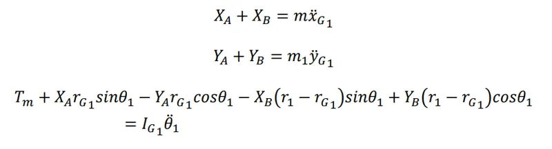
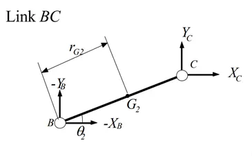
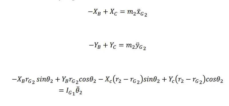
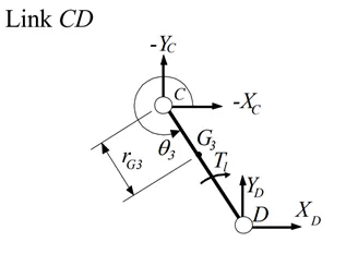
The force as well as the torque acting in both XY direction in links AB ,BC,CD need to be calculate dindividually to carry out a dynamic analysis.

Dynamic analyis for link AB

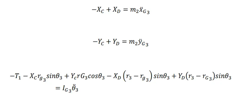
Dynamic analysis for link BC

Dynamic analysis for link CD

CODING

% SUBMITTED BY VIKAS
% FINAL INDEPENDENT PROJECT 
% MATEHEMATICAL ANALYSIS , VELOCITY ANALYSIS ,ACCELERATION ANALYSIS ,
% DYNAMIC ANALYSIS OF FOUR BAR MECHANISM

% VARIABLE INPUT
r1=0.01; 
r2=0.035; 
r3=0.02; 
r4=0.03;
rg1=r1/2; 
rg2=r2/2;
rg3=r3/2; 

ig1=0.00002; 
ig2=0.0005;
ig3=0.00009;

w1=100;

m1=0.3;
m2=0.5; 
m3=0.6; 
a1=0; 
i=0; 

for TH1=0:0.001:2*pi

 A=cos(TH1)-(r4/r1);
 B=sin(TH1);
 C=(r4/r3)*cos(TH1)-((r1^2-r2^2+r3^2+r4^2)/(2*r1*r3));
 R=sqrt(A^2+B^2);
 Z=C/R;
 zz=sqrt(1-Z^2);
 i=i+1;

% POSITION ANALYSIS

TH3=atan2(B,A)+atan2(zz,Z);
if TH3<0; TH3=TH3+2*pi;end

TH3b=atan2(B,A)-atan2(zz,Z);
if TH3b<0; TH3b=TH3b+2*pi;end

TH2=atan2((-r3*sin(TH3)-r1*sin(TH1)),(r4-r3*cos(TH3)-r1*cos(TH1)));

T1(i)=TH1; T2(i)=TH2; T3(i)=TH3; T3b(i)=TH3b;

% VELOCITY ANALYSIS

w3=w1*(r1*sin(TH1-TH2))/(r3*sin(TH2-TH3));
w2=w1*(r1*sin(TH3-TH1))/(r2*sin(TH2-TH3));

W3(i)=w3; W2(i)=w2;

% ACCELERATION ANALYSIS

a3=(w1^2*r1/r3)*((1-(w2/w1))*cos(TH1-TH2)*sin(TH2-TH3)-((w2/w1)-(w3/w1))*cos(TH2-TH3)*sin(TH1-TH2))/(sin(TH2-TH3))^2;
a2=-(w1^2*r1/r2)*((1-(w3/w1))*cos(TH1-TH3)*sin(TH2-TH3)-((w2/w1)-(w3/w1))*cos(TH2-TH3)*sin(TH1-TH3))/(sin(TH2-TH3))^2;

A3(i)=a3; A2(i)=a2;


% ACCELERATION G1 G2 G3
xg1= -rg1* (a1*sin(TH1) +w1^2*cos (TH1)); 
yg1= rg1* (a1*cos (TH1) -w1^2*sin (TH1));

xg2= -r1* (a1*sin (TH1) +w1^2*cos (TH1))- rg2* (a2*sin (TH2) +w2^2*cos(TH2)); 
yg2= r1* (a1*cos (TH1) -w1^2*sin (TH1))+ rg2* (a2*cos (TH2)-w2^2*sin (TH2));

xg3= (r3-rg3)*(a3*sin(TH3)+w3^2*cos(TH3));
yg3= -(r3-rg3)*(a3*cos(TH3)-w3^2*sin(TH3));

% DYNAMIC ANALYSIS
A=[1 0 1 0 0 0 0 0 0;
   0 1 0 1 0 0 0 0 0; 
   rg1*sin(TH1) -rg1*cos(TH1) -(r1-rg1)*sin(TH1) (r1-rg1)*cos(TH1) 0 0 0 0 1; 
   0 0 -1 0 1 0 0 0 0; 
   0 0 0 -1 0 1 0 0 0; 
   0 0 -rg2*sin(TH2) rg2*cos(TH2) -(r2-rg2)*sin(TH2) (r2-rg2)*cos(TH2) 0 0 0; 
   0 0 0 0 -1 0 1 0 0;
   0 0 0 0 0 -1 0 1 0; 
   0 0 0 0 -rg3*sin(TH3) rg3*cos(TH3) -(r3-rg3)*sin(TH3) (r3-rg3)*cos(TH3) 0];


B =[ m1*xg1;
     m1*yg1; 
     ig1*a1; 
     m2*xg2; 
     m2*yg2; 
     ig2*a2; 
     m3*xg3;
     m3*yg3; 
     ig3*a3];


X=inv(A)*B ;
XA (i)=X(1,1);
YA (i)=X(2,1);
XB (i)=X(3,1);
YB (i)=X(4,1);
XC (i)=X(5,1);
YC (i)=X(6,1);
XD (i)=X(7,1);
YD (i)=X(8,1);
TM (i)=X(9,1);

end

% PLOTTING
% PLOT OF JOINT A
figure (1)
plot (XA, YA,'LineWidth',3,'color','r') 
grid
title ('POLAR LOAD  FOR JOINT A') 
xlabel('Fx,N') 
ylabel('Fy,N'); 


% PLOT OF JOINT B 
figure (2) 
plot (XB, YB,'LineWidth',3,'color','b') 
grid 
title('POLAR LOAD FOR  JOINT B') 
xlabel('Fx,N') 
ylabel('Fy,N'); 


% PLOT OF JOINT C 
figure (3) 
plot (XC, YC,'LineWidth',3,'color','g')
grid
title('POLAR LOAD FOR JOINT C') 
xlabel('Fx,N') 
ylabel('Fy,N'); 


% PLOT OF JOINT D 
figure (4) 
plot (XD, YD,'LineWidth',3,'color','y')
grid
title('POLAR LOAD FOR JOINT D') 
xlabel('Fx,N') 
ylabel('Fy,N'); 

% PLOT OF MOTOR TORQUE
figure (5) 
plot (T1*180/pi,TM,'LineWidth',3,'color','b')
grid
title('VARIATION OF MOTOR TORQUE') 
xlabel('\Theta 1,deg') 
ylabel('Tm,N.m'); 

Variable input

% VARIABLE INPUT
r1=0.01; 
r2=0.035; 
r3=0.02; 
r4=0.03;
rg1=r1/2; 
rg2=r2/2;
rg3=r3/2; 

ig1=0.00002; 
ig2=0.0005;
ig3=0.00009;

w1=100;

m1=0.3;
m2=0.5; 
m3=0.6; 
a1=0; 
i=0; 

for TH1=0:0.001:2*pi

 A=cos(TH1)-(r4/r1);
 B=sin(TH1);
 C=(r4/r3)*cos(TH1)-((r1^2-r2^2+r3^2+r4^2)/(2*r1*r3));
 R=sqrt(A^2+B^2);
 Z=C/R;
 zz=sqrt(1-Z^2);
 i=i+1;

Position Analysis

% POSITION ANALYSIS

TH3=atan2(B,A)+atan2(zz,Z);
if TH3<0; TH3=TH3+2*pi;end

TH3b=atan2(B,A)-atan2(zz,Z);
if TH3b<0; TH3b=TH3b+2*pi;end

TH2=atan2((-r3*sin(TH3)-r1*sin(TH1)),(r4-r3*cos(TH3)-r1*cos(TH1)));

T1(i)=TH1; T2(i)=TH2; T3(i)=TH3; T3b(i)=TH3b;

Velocity Analysis

% VELOCITY ANALYSIS

w3=w1*(r1*sin(TH1-TH2))/(r3*sin(TH2-TH3));
w2=w1*(r1*sin(TH3-TH1))/(r2*sin(TH2-TH3));

W3(i)=w3; W2(i)=w2;

Acceleration Analysis

% ACCELERATION ANALYSIS

a3=(w1^2*r1/r3)*((1-(w2/w1))*cos(TH1-TH2)*sin(TH2-TH3)-((w2/w1)-(w3/w1))*cos(TH2-TH3)*sin(TH1-TH2))/(sin(TH2-TH3))^2;
a2=-(w1^2*r1/r2)*((1-(w3/w1))*cos(TH1-TH3)*sin(TH2-TH3)-((w2/w1)-(w3/w1))*cos(TH2-TH3)*sin(TH1-TH3))/(sin(TH2-TH3))^2;

A3(i)=a3; A2(i)=a2;


% ACCELERATION G1 G2 G3
xg1= -rg1* (a1*sin(TH1) +w1^2*cos (TH1)); 
yg1= rg1* (a1*cos (TH1) -w1^2*sin (TH1));

xg2= -r1* (a1*sin (TH1) +w1^2*cos (TH1))- rg2* (a2*sin (TH2) +w2^2*cos(TH2)); 
yg2= r1* (a1*cos (TH1) -w1^2*sin (TH1))+ rg2* (a2*cos (TH2)-w2^2*sin (TH2));

xg3= (r3-rg3)*(a3*sin(TH3)+w3^2*cos(TH3));
yg3= -(r3-rg3)*(a3*cos(TH3)-w3^2*sin(TH3));

Matrix for Dynamic analysis

Matrix can be now be used to solve the dynamic equation used above . The matrix will be written

[A]*[B]=[X]

Where

A= is the multiplying variable of the instantaneous geomerty of the mechanism

B= is the multiplying variable defines the velocity and acceleration links

X= The sum of the multiplying variables A and B where the plot for the MATLAB  results will be obtained

Dynamic Analysis

% DYNAMIC ANALYSIS
A=[1 0 1 0 0 0 0 0 0;
   0 1 0 1 0 0 0 0 0; 
   rg1*sin(TH1) -rg1*cos(TH1) -(r1-rg1)*sin(TH1) (r1-rg1)*cos(TH1) 0 0 0 0 1; 
   0 0 -1 0 1 0 0 0 0; 
   0 0 0 -1 0 1 0 0 0; 
   0 0 -rg2*sin(TH2) rg2*cos(TH2) -(r2-rg2)*sin(TH2) (r2-rg2)*cos(TH2) 0 0 0; 
   0 0 0 0 -1 0 1 0 0;
   0 0 0 0 0 -1 0 1 0; 
   0 0 0 0 -rg3*sin(TH3) rg3*cos(TH3) -(r3-rg3)*sin(TH3) (r3-rg3)*cos(TH3) 0];


B =[ m1*xg1;
     m1*yg1; 
     ig1*a1; 
     m2*xg2; 
     m2*yg2; 
     ig2*a2; 
     m3*xg3;
     m3*yg3; 
     ig3*a3];


X=inv(A)*B ;
XA (i)=X(1,1);
YA (i)=X(2,1);
XB (i)=X(3,1);
YB (i)=X(4,1);
XC (i)=X(5,1);
YC (i)=X(6,1);
XD (i)=X(7,1);
YD (i)=X(8,1);
TM (i)=X(9,1);

end

Plotting

% PLOTTING
% PLOT OF JOINT A
figure (1)
plot (XA, YA,'LineWidth',3,'color','r') 
grid
title ('POLAR LOAD  FOR JOINT A') 
xlabel('Fx,N') 
ylabel('Fy,N'); 


% PLOT OF JOINT B 
figure (2) 
plot (XB, YB,'LineWidth',3,'color','b') 
grid 
title('POLAR LOAD FOR  JOINT B') 
xlabel('Fx,N') 
ylabel('Fy,N'); 


% PLOT OF JOINT C 
figure (3) 
plot (XC, YC,'LineWidth',3,'color','g')
grid
title('POLAR LOAD FOR JOINT C') 
xlabel('Fx,N') 
ylabel('Fy,N'); 


% PLOT OF JOINT D 
figure (4) 
plot (XD, YD,'LineWidth',3,'color','y')
grid
title('POLAR LOAD FOR JOINT D') 
xlabel('Fx,N') 
ylabel('Fy,N'); 

% PLOT OF MOTOR TORQUE
figure (5) 
plot (T1*180/pi,TM,'LineWidth',3,'color','b')
grid
title('VARIATION OF MOTOR TORQUE') 
xlabel('\Theta 1,deg') 
ylabel('Tm,N.m'); 

Results

                     

                

            

                                         

                          

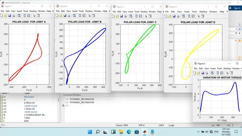
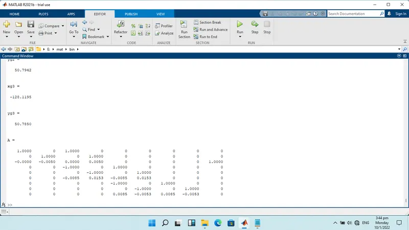
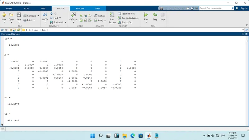
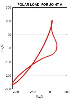
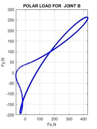
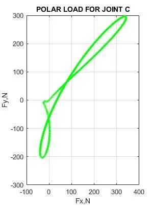
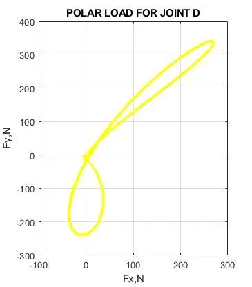
Figure shows Polar Loads of joints A,B,C D is the results of the dynamic analysis of all force s. It is apparent A and B a very similar in creating perhaps most joints having the same magnitude while moving the constant velocity. The same can be said for joints C and D

                                                                       

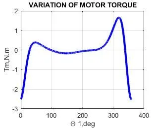
Variation when the torque is applied to joints A  and B . At each cycle of the mechanism there is an increase in the torque of the motor and the angular velocity is constant . As the link moves energy is stored in th elink and when the energy generated from the torque of the motor is zero the energy stored in the link returns to the motor and vice versa . This explains the fluctiation of the peaks shows for torque above

 CONCLUSION

With the help of MATLAB software we analysed the velocity and postion , accleration, dynamics analysis and ploted graph of four bar and two bar mechanism.

Four Bar linkages can be used for many mechanical purposes including to convert rotational to reciprocating motion.