FINAL INDEPENDENT PROJECT

1. Aim:

To demonstrate the physical working of the dynamic bicycle model under a "Perturbation" dynamics using Matlab.

2. Principle Description:

2.1 The Dynamic Bicycle Model:

2.1.1 Parameters:

• m: Vehicle mass.
• `I_z`: Moment of Inertia of the vehicle about the z-axis.
• r: Yaw rate.
• `l_f , l_r`: Distance of CG to front and rear axle.
• V: Magnitude of vehicle's longitudinal velocity.
• `beta`: Magnitude of vehicle's lateral velocity.
• `C_f, C_r`: Cornering stiffness of front and rear tyres.

2.1.2 Assumptions:

• Left and Right wheels are lumped together.
• The local reference frame is kept at the vehicle's CG.
• The vehicle's motion is restricted in x-y plane.
• Vehicle velocity is constant and tangent to the circular path and at any instance, the path remains a section of a perfect circle.
• The steering angle of vehicle is small such that: `sin(delta)~delta; cos(delta)~1; tan(delta)=delta`.

2.1.3 Equations of Motion:

There are two kinds of equations upon which the complete model is based:

• Force Equation: `=> sum F=m*a....(1)`
• Moment Equation: `=> sum M=I_z*dot r....(2)`

Where,

`F->`Forces in x-y plane on the body.

`M->`Moments in x-y plane.

`a->`Acceleration of the CG with respect to inertial frame.

`dot r->`Yaw rate of the vehicle.

Resolving front and rear tyre forces on the body frame of reference: `F_f + F_r=m*a....(1)`

Acceleration: `=> a=V*(dot beta+r)` (simplified from assumption)

Thus, eq(1) becomes: `=> F_r+F_f=m*(V*(dot beta+r))`

Now, as we take moment about the CG, we get the modified eq(2): `=> I_z*dot r=F_f*l_f + F_r*l_r`

2.1.4 Tyre Model:

We now have vehicle forces but in order to capture the complete vehicle motion, we must encorporate tyre forces as well. A popular model which is widely used in industries, is the Pacejka Tyre Model, an imperical model which assumes several constants based on various testing results that capture the tyre forces very accurately. This model takes most situations into account within the tyre's performance range.

However, for a simplified bicycle model simulation, we can easily get by with a linear tyre model which surprisingly, gives results very close to the experimental range.

Note: The linear tyre model computes `F_y` and `alpha` in the linear range for the imperical tyre model.

`=> C_alpha=-[(del F_y)/(del alpha)]_(alpha=0)`

for small slip angles, i.e.: `alpha in` -3 to +3 degrees, the lateral force is approximated by:

`=> F_y=-C_alpha*alpha` where, for right turn, `alpha=>`positive and for left turn, `alpha=>`negative.

`=> F_(yf)=-C_f*alpha_f` for front and,

`=> F_(yr)=-C_r*alpha_r` for the rear.

Note: These `C(f,r)` values are for a set of tyres (left and right) and must be halved to find stiffness of a single tyre.

Using geometry, we can find out `alpha_f` and `alpha_r`:

`=> alpha_f=beta+((r*l_f)/V)-delta` for front and,

`=> alpha_r=beta-((r*l_r)/V)` for rear.

Now, if we back-substitute these in the linear tyre model equation, we get:

Front Tyre Force`=> F_f=-C_f*(beta+(r*l_f)/v-delta)`

Rear Tyre Force`=> F_r=-C_r*(beta-(r*l_r)/V)`

2.1.5 Simplifying and Analysing:

As we back-substitute these force values in equations (1) and (2), we get:

`=> m*V(dot beta+r)=C_r*((r*l_r)/V-beta)+C_f*(delta-beta-(r*l_f)/V)`

`=>-(C_r+C_f)*beta+r/V*(C_r*l_r-C_f*l_f)+C_f*delta`

This equation is a sum of three factors:

1. The damping in side slip derivative `Y_beta=-(C_r+C_f)`, describing the amount of damping generated per side-slip angle (always negative). This acts as a damper resisting the side slip.
2. The yaw coupling derivative `Y_r=1/V(C_r*l_r-C_f*l_f)`, describing the amount of lateral force generated with increase in yaw rate (can be positive or negative). This gets smaller with increasing velocity.
3. The control force derivative `Y_delta=C_f`(for front-steered vehicle), describing the lateral force generated per steer angle.

Similarly, equation(2) becomes:

`=> I_z*dot r=l_f*C_f*(delta-beta-(r*l_f)/V)-l_r*C_r*((r*l_r)/V-beta)`

`=> (C_r*l_r-C_f*l_f)*beta-r/V(C_f*l_f^2+C_r*l_r^2)+C_f*l_f*delta`

This equation as well is a sum of three factors:

1. The Directional Stability Derivative `N_beta=C_r*l_r-C_f*l_f`, describing the yaw moment produced per side slip angle (can be +ve/-ve/0). This factor is key in determining the nature of steering of the vehicle (-ve: Oversteer/+ve: Understeer/0: Neutral Steer).
   
2. The Yaw-Damping Derivative `N_r=-1/V(C_f*l_f^2+C_r*l_r^2)`, describing the effect of yaw rate on yaw moment. This produces a moment that acts like a damper trying to resist change in yaw rate, making the car directionally stable. This term decreases with increasing speeds i.e. at higher speeds, small perturbations result in a change that is difficult to correct.
3. The Control Moment Derivative `N_delta=C_f*l_f`, describing the effect of yaw moment, this value increases with front cornering stiffness and/or as the CG moves rearwards.

2.1.6 Bringing everything together:

The two equations have now become:

`=> m*V*(dot beta+r)=Y_beta*beta+Y_r*r+Y_delta*delta`

`=> dot beta=((Y_beta*beta)/(m*V))+((Y_r*r)/(m*V))+((Y_delta*delta)/(m*V))-r`

`=> dot beta= ((Y_beta*beta)/(m*V))+((Y_delta*delta)/(m*V))+((Y_r)/(m*V)-1)*r....(1)` and

`=> I_z*dot r=N_beta*beta+N_r*r+N_delta*delta....(2)`

Combining (1) and (2):

`[(dot beta),(dot r)]=[[(Y_beta/(m*V)) (Y_r/(m*V)-1)],[(N_beta/I_z) (N_r/I_z)]]*[(beta),(r)]+[(Y_delta/(m*V)),(N_delta/I_z)]*delta`

3. Objective:

This project aims to demonstrate the steady-state analysis of a vehicle which examins a fixed state a vehicle reaches eventually when given a fixed steering input and then capture these motion snapshots through a time window. Along with these, the vehicle path and side slip angles will also be demonstrated through the same time window.

4. Code:

4.1 Passenger Car Parameters:

m=1500;             %[kg]
Iz=2873;            %[kg*m^2]
L=2.68;             %[m]
WF=0.59;            %[ratio %]
Lr=WF*L;            %[dist from CG to rear axle]
Lf=L-Lr;            %[dist from CG to front axle]
Cf=80000;           %[N/rad(Combined FRONT)]
Cr=Cf;              %[N/rad(Combined REAR)]
Rt=0.26;            %[m (tyre radius)]

Vkmph=80;           %[constant velocity in kmph]
V=Vkmph*0.277778;   %[constant velocity in m/s]

4.2 Simplifying Factors:

Ybeta= -(Cr+Cf);    %[damping in sideslip derivative]
Yr=(Cr*Lr-Cf*Lf)/V; %[yaw coupling derivative]
Ydelta=Cf;          %[control force derivative]
Nbeta=Cr*Lr-Cf*Lf;  %[directional stability derivative]
Nr=-(Cf*Lf^2+Cr*Lr^2)/V; %[yaw damping derivative]
Ndelta=Cf*Lr;       %[control moment derivative]

4.3 State-Space form and Steering Input with time vector definition:

By Euler forward integration:

`[[beta(t+trianglet)],[r(t+trianglet)]]=[[beta(t_0)],[r(t_0)]]+[[dot beta(t_0)],[dot r(t_0)]]*trianglet`

Note: Here, `omega` is the frequency of applied sinusoidal steering input.

A=[Ybeta/(m*V), Yr/(m*V)-1;...
    Nbeta/Iz, Nr/Iz];
B=[Ydelta/(m*V);...
    Ndelta/Iz]; 

beta0=0;            %initial side slip angle
r0=0;               %initial yaw rate

states(:,1)=[beta0,r0];

dt=0.01;
t=(0:dt:10)';
N=length(t);
T=10;
omega=2*(2*pi/T);
delta=10*pi/180*sin(omega*t);
dstates(:,1)=A*states(:,1)+B*delta(1);

for k=1:N-1
    
    dstates(:,k)=A*states(:,k)+B*delta(k);
    states(:,k+1)=states(:,k)+dstates(:,k)*dt;
    
end

beta=states(1,:);
r=states(2,:);

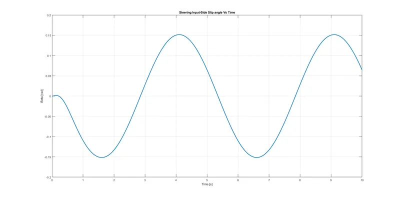
figure(1)
plot(t,beta,'linewidth',2),grid on
xlabel('Time [s]'),ylabel('Beta [rad]')
title('Steering Input-Side Slip angle Vs Time')

4.4 Path prediction given `beta` and r:

Heading angle: `=> dot psi equiv r`

`=> psi(t_0+triangle t)=psi(t_0)+r(t_0)*triangle t`

we are interested to find (x,y) relative to our fixed frame:

`=> x(t_0+trianglet)=x(t_0)+V_x(t_0)*trianglet`

`=> y(t_0+trianglet)=y(t_0)+V_y(t_0)*trianglet`

At any time instant,

`V_x=cos(psi+beta)` and `V_y=V*sin(psi+beta)`

psi(1)=0;
x(1)=0;
y(1)=0;
for k=1:N-1
    psi(k+1)= psi(k)+r(k)*dt;
    
    Vx(k)=V*cos(psi(k)+beta(k));
    Vy(k)=V*sin(psi(k)+beta(k));
    
    x(k+1)=x(k)+Vx(k)*dt;
    y(k+1)=y(k)+Vy(k)*dt;
end

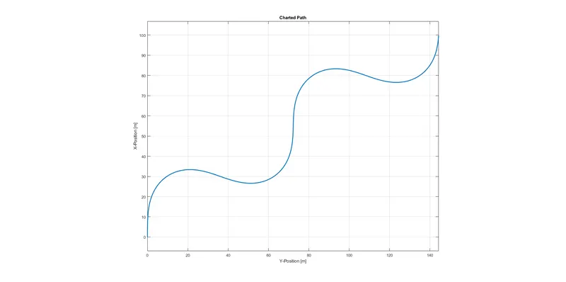
figure(2)
plot(y,x,'linewi',2),grid on
xlabel('Y-Position [m]'),ylabel('X-Position [m]')
title('Charted Path')
axis equal

4.5 Animating Vehicle as a function of time:

• CG Position: `(x,y)`
• Front Wheel Position: `(x+l_f*cos(psi)),(y+l_f*sin(psi))`
• Rear Wheel Position: `(x-l_r*cos(psi)),(y-l_r*sin(psi))`
• Specific Co-ordinates, example- Front of Front Tyre: `(x_f+R_t*cos(psi+delta)),(y_f+R_t*sin(psi+delta))`

xF = x + Lf*cos(psi);
yF = y + Lf*sin(psi);
xR = x - Lr*cos(psi);
yR = y - Lr*sin(psi);

xF_F=xF+Rt*cos(psi+delta');           %x-pos front of front tyre
yF_F=yF+Rt*sin(psi+delta');           %y-pos front of front tyre
xF_R=xF-Rt*cos(psi+delta');           %x-pos rear of front tyre
yF_R=yF-Rt*sin(psi+delta');           %y-pos rear of front tyre

xR_F=xR+Rt*cos(psi);                  %x-pos front of rear tyre
yR_F=yR+Rt*sin(psi);                  %y-pos front of rear tyre
xR_R=xR-Rt*cos(psi);                  %x-pos rear of rear tyre
yR_R=yR-Rt*sin(psi);                  %y-pos rear of rear tyre

skip=2;

for k=1:skip:N

    figure(3)

    plot(y(1:k),x(1:k),'c-','linewi',2);grid on; hold on; 
    plot([yF_R(k) yF_F(k)],[xF_R(k) xF_F(k)],'r-','linewidth',6);
    plot([yR_R(k) yR_F(k)],[xR_R(k) xR_F(k)],'r-','linewidth',6);
    plot(y(k),x(k),'ko','markersize',6,'linewidth',4);
    plot([yR(k) yF(k)],[xR(k) xF(k)],'k-','linewidth',4);hold off;
    axis equal
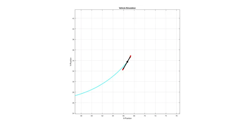
    title('Vehicle Simulation')
    xlabel('X-Position')
    ylabel('Y-Position')

    %axis limits:([LEFT RIGHT BOTTOM TOP])
    axis([y(k)-Lf*9 y(k)+Lf*9 x(k)-Lf*9 x(k)+Lf*9]) 

    drawnow
end

5. Results:

5.1 Side Slip Vs Time: Modify 'delta', 'omega' and time period value to change.

5.2 Charted vehicle path: Dependant on 'beta' and 'r' which in turn, depends on 'delta'.

5.3 Instantaneous vehicle position (Random Instant): Bicycle constructed using simple lines and using angle 'psi' as an input as it changes with each step.

6. Future Scope & Conclusion:

Using the equations:

`=> m*V*(dot beta+r)=Y_beta*beta+Y_r*r+Y_delta*delta` and,

`=> I_z*dot r=N_beta*beta+N_r*r+N_delta*delta`

..the following question could be answered:

Given a steering angle, say `delta=1` degree, what will be the vehicle's steady state lateral acceleration, side slip angle and yaw rate? Also, how much lateral force is produced at front vs rear tyres?

This could be answered by integrating the bicycle equation over time and examining the steady-state values that the parameters approach. A transient response (i.e. how dynamics vary with time as steering inputs are applied) takes place in the settling time after which a steady-state response is shown.

However, using the final value theorem, we can derive an expression for each of these steady-state values. These will give us insights to how different vehicle parameters affect the response.

Most important parameters are: front weight distribution and front Vs rear tyre cornering stiffness.

6.1 Final Value Theorem:

`lim_(t->oo) f(t)=lim_(s->0) s*f(S)` where,

`f(S)=Laplace{f(t)}` and `S` is the complex independantvariable of domain `s`.

When we calculate the Laplace transforms of the two functional equations above and solve for `beta(S)` and `r(S)`, we will find two transfer functions which woud relate steering input to side-slip angle and yaw rate respectively. We can then apply the Final Value Theorem to these expressions to find the steady state side slip angle or yaw rate when steering angle is set to some value.

When we calculate the value of lateral acceleration, instantaneous slip angle and the tyre forces, we would discover that the front tyre is doing more work when making a particular maneuver within a certain range of steering input and CG location. This means that under extreme conditions, the front would give out before the rear does and this is a safe design strategy.

The two main factors contributing to this safe characterstic in a real world are:

1. Tyre tread design.
2. Overall weight distribution of the vehicle.

Key Takeaway: When a vehicle runs through a course, it really is transitioning between different steady-state conditions while driving.

7. Sources:

1. Matlab plot Help
2. Tyre Co-ordinate sysyem (reference): Tire Axis System YT.
3. Tyre Model (Pacejka): Magic Formula.
4. Final Value Theorem (for further evaluation): Final Value Theorem.
5. SHM YouTube: Physical Models+ Differential Equations.
6. Euler Forward: Wikipedia for Euler Method.