Week 4.1 - Genetic Algorithm

Aim:

1. To write a Matlab Script which optimizes the stalagmite function and also returns the global maxima of the function.
2. To present a thorough discussion on the principle of GA(Genetic Algorithm) and how its useful in programming today along with the ga syntax in Matlab.
3. The written script should give the same output even if its made to run several times.

Description:

Genetic Algorithm is a procedure of selecting a sample of multiple prototypes(could be datapoints, could even be real world objects) and coming up with the most fit result. A 'fit' result would be the value of datapoints which is the closest to the actual best result. A typical Genetic Algorithm requires:

1. A Genetic Representation of the solution domain.
2. A Fitness function to evaluate the solution domain.
3. Apart from these, the full procedure of GA also requires:
   i. A function to generate new solutions. ii. A selection function iii. A crossover function and iv. A mutation function.

In order to make this process even clearer, lets looks at the process flow for GA with the knapsack example:

Imagine a condition where we are required to pack a bagpack for a trip such that a certain weight limit is not exceeded. In this first sentence, the highlighted text is a problem task or a 'Fitness Function'.

Note: In this example, there are clearly more fitness functions required for the sake of a near-perfect result. However, for the sake of example, it easily gets the point across and hence there is just one fitness function here.

A Fitness Function is nothing but a simple rule or set of rules that govern the 'goodness of a result'. From our small list on the requirements for evaluating a GA, this is the second part.

Coming back to the bagpack. Let's assume we have prepared a list of items to be kept in the bagpack and in an ideal case, we would want everything in the bagpack but then it would violate the rules set by our fitness function by crossing the weight limit. Hence, we're better off by leaving this problem to the GA which simply works on 'survival of the fittest'.

Now lets assume we have prepared a list of 10 items amongst which we're interested to find the best possible fit.

Finally, we will get to the first requirement of conducting a GA, coming up with a genetic representation. By using binary, we can define what combinations to use, if an item gets a 1, it goes in the bagpack but if an item gets a 0, it stays out. The process of GA always starts with a random population description and this first set of combinations is called the Generation 0.

Now that both the requirements have been met, we can start with the process of natural selection in order to come up with the best possible solution. In this step, the fitness function will play a significant role.

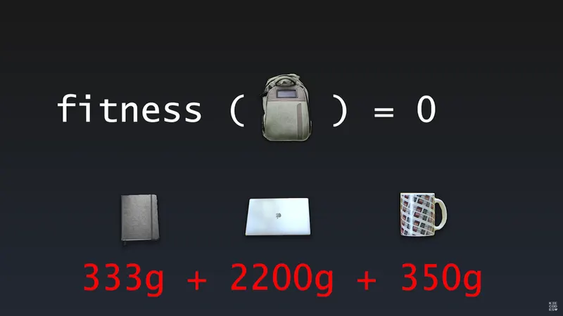
Hence, if in any particular case, the fitness function is not satisfied, the function value equates to zero and that particular condition is considered the worst, similarly, from the Generation 0, two best cases are more likely to be picked to then come up with another combination(Single-point Crossover function: the genome of the two parents are cut at the same point and is interchanged) this combination is better than the best of Generation 0 and is hence a part of Generation 1. This process is repeated until we don't have enough specimens in the next generation.

As both the process of selection and crossover are governed by randomness, we perform illitism which is simply picking 'n' top cases from the previous generation and transferring them to the next generation.

At this stage it's time to introduce a mutation where we simply randomly change a bit of the genome of each element

Therefore, with each step, this process results in better and better results until however, it reaches a point of saturation after which the results of every consecutive generation does not differ by a significant amount, this is the point where we stop the iterations.

Syntax for GA in Matlab: Given Below is the full syntax of GA in matlab-

[input,fval]=ga(fitnessfn,nvars,A,B,Aeq,Beq,LB,UB,nonlcon,IntCon,options)

where:

Item	Description
input	returns the input values.
fval	returns the value of the fitness function.
fitnessfn	the function which we desire to minimize.
nvars	the number of variables associated with the function.
A & B	linear inequality constrains of type `A*x<=B` if any.
Aeq & Beq	equality constrain of the type `A*x=B` if any.
LB & UB	these define the upper and lower bounds of the function and these constrain GA in the desired domain.
nonlcon	defines a non-linear constrain if any.
IntCon	defines an integer constrain if any.
options	these provide further modifications(ex: populationSize).

Note: The above table highlights all the values that are associated with a typical GA-defining line of code. All of these values are rarely ever required altogether in a way represented above. However, the user needs to account for the spaces that each of these values hold and thus must make sure that the spaces are filled by [ ] in order to account for a null value for that particular aspect as will be represented in this report later.

Stalagmite Function: In order to execute this task, the following stalagmite function will be used:

`f=f_x*f_y*g_x*g_y;` where:

`f_x=[sin(5.1*pi*x+0.5)]^6;`

`f_y=[sin(5.1*pi*y+0.5)]^6;`

`g_x=exp[-4*ln(2)*(x-0.0667)^2/0.64];`

`g_y=exp[-4*ln(2)*(y-0.0667)^2/0.64]`

Code:

Stalagmite Function: The Stalagmite function is our governing Fitness Function which ensures the construction of the entire surface plot and the stalagmite function is the same function that we aim to optimize in order to return consistent values for the global maxima. This will be accounted for in our main script.

function [P]=stalagmite (ip_vector)
    x=ip_vector(1);
    y=ip_vector(2);
    fx=(sin(5.1*pi*x+0.5))^6;
    fy=(sin(5.1*pi*y+0.5))^6;
    gx=exp((-4*log(2)*((x-0.0677)^2)/0.64));
    gy=exp((-4*log(2)*((y-0.0677)^2)/0.64));
    P=-1*(fx*fy*gx*gy);
end   

Calling Stalagmite function in order to visually check the actual global maxima:

Auxiliary Code:

Defining Search Space-

x=linspace(0,0.6,150);
y=linspace(0,0.6,150);

Creating 2-D mesh-

[xx, yy]=meshgrid(x,y);

Evaluating Stalagmite function:

for i=1:length(xx)
    for j= 1:length(yy)
        ip_vector(1)=xx(i,j);
        ip_vector(2)=yy(i,j);
        f(i,j)=stalagmite(ip_vector);
    end
end

Plotting results:

surfc(xx,yy,f)
shading interp
[inputs, fval]=ga(@stalagmite,2);
xlabel('x-val')
ylabel('y-val')
zlabel('peak magnitude')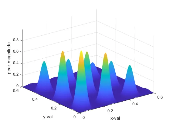

This leads us onto our main script where we integrate all these properties along with our stalagmite function:

Main Script: This script is split into three distinct modes of study which are nothing but different approaches to get a better result such that each study displays a better result over the previous one.

Evaluating Stalagmite function:

clear
close all
clc

x=linspace(0,0.6,150);
y=linspace(0,0.6,150);
num_cases=50;

% Creating 2D mesh
[xx, yy]=meshgrid(x,y);

% Evaluating Stalgamite Function
for i=1:length(xx)
    for j= 1:length(yy)
        ip_vector(1)=xx(i,j);
        ip_vector(2)=yy(i,j);
        f(i,j)=stalagmite(ip_vector);
    end
end

surfc(xx,yy,f)

shading interp
[inputs, fval]=ga(@stalagmite,2);
xlabel('x-val')
ylabel('y-val')
zlabel('peak magnitude')

Study-1: Statistical Behaviour

tic
for i=1:num_cases
    [inputs,fopt(i)]=ga(@stalagmite,2); 
    xopt(i)=inputs(1);
    yopt(i)=inputs(2);
end
study1_time=toc;
figure(1)
subplot(2,1,1)
hold on
surfc(x,y,f)
shading interp
plot3(xopt,yopt,fopt,'marker','o','markersize',5,'markerfacecolor','r')
title('Study-1: Unbounded Inputs')
subplot(2,1,2)
plot(fopt)
xlabel('Iterations')
ylabel('Function Maximium')

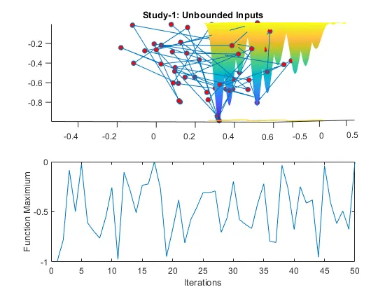
Study-1 Result: As seen from the figure below, the obtained values are scattered all over the graph which is not really useful.

Study-2: The problems faced while plotting could be limited by setting the upper and lower bounds to our function search space.

Note: the commands given below are our target search space but, GA does not recognize this and in order to make a correction, we need to include these upper and lower bounds in the GA call itself(refer to GA syntax).

x=linspace(0,0.6,150);
y=linspace(0,0.6,150);

Study-2: Including upper and lower bounds.

tic
for i=1:num_cases
    [inputs,fopt(i)]=ga(@stalagmite,2,[],[],[],[],(0:0),(0.6:0.6));
    xopt(i)=inputs(1);
    yopt(i)=inputs(2);
end
study2_time=toc;
figure(2)
subplot(2,1,1)
hold on
surfc(x,y,f)
shading interp
plot3(xopt,yopt,fopt,'marker','o','markersize',5,'markerfacecolor','g')
title('Study-2: Unbounded Inputs')
subplot(2,1,2)
plot(fopt)
xlabel('Iterations')
ylabel('Function Maximium')

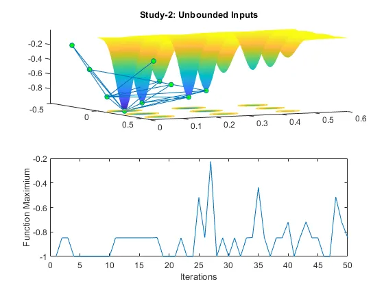
Study-2 Result: As we see from the figure below, the search space is somewhat refined and the picked values are within the required bounds. However, we are not quite there yet as GA still predicts several values outside our desired range.

Study-3: In order to improve the results further, we need to revisit the concept of GA where it says that the results do tend to improve with an increased population size. Now by default, GA takes a population size of 50 which produces these results. in this part we will upscale the population in order to bring improvements to our results.

options=optimoptions('ga');
options=optimoptions(options,'PopulationSize',170);
tic
for i=1:num_cases
    [inputs,fopt(i)]=ga(@stalagmite,2,[],[],[],[],(0:0),...
        (0.6:0.6),[],[],options);
    xopt(i)=inputs(1);
    yopt(i)=inputs(2);
end
study3_time=toc;
figure(3)
subplot(2,1,1)
hold on
surfc(x,y,f)
shading interp
plot3(xopt,yopt,fopt,'marker','o','markersize',5,'markerfacecolor','k')
title('Study-3: Bounded Inputs+ Modified Population size')
subplot(2,1,2)
plot(fopt)
xlabel('Iterations')
ylabel('Function Maximium')

Here, we have brought the population size along with positive changes from Study-2 together to get the following result:

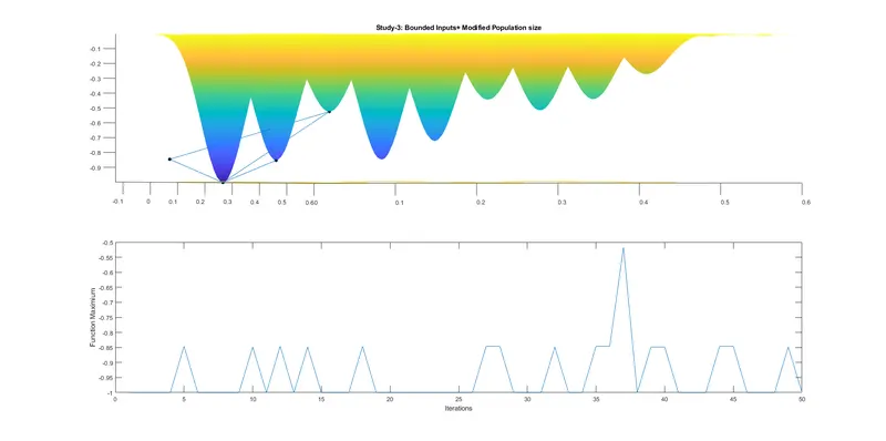
As seen from the graph thus obtained, the rerults are far more satisfactory.

Evidently, as the subsequent cases are more and more refined, they take more time to execute. In order to visualize that, heres a few lines that can be added at the end:

Note: Time is in seconds.

STtime=[study1_time,study2_time,study3_time];
studyserial=[1,2,3];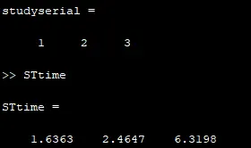

Conclusion:

Hence, by step by studying GA thoroughly and by encorporating the rules of GA accordingly, we were ale to optimize the stalagmite function and also locate the global maxima appropriately.

Note: As the GA is only used to maximize a function, we inversed the minimum function itself in the function definition.

Sources:

1. Wikipedia: GA Info.
2. Youtube Video for GA: YouTube-GA.
3. GA help in matlab for GA syntax.
4. GA and stalagmite function: GA+Stalagmite.