Week 3 - Solving second order ODEs

Aim:

1. To present a code that outputs the motion of a pendulum similar to the sample GIF following the given ODE:
   `d^2/dt^2(theta)+(b/m)*d/dt(theta)+(g/l)*sin theta=0`
2. To capture this motion in a video file.

Governing Equation:

A differential equation is the most straightforward way to represent any process that occours in the real world, and in case of representing the motion of a simple pendulum in this case, we need to compute values of the displacement and velocity as they are the two variables which would give us a proper description of the given second order ODE.

Although, in order to solve this equation, we first need to break it down into two-first order equations and solve them individually.

Note: The order of simplification and the definative variables, both are equal to the order of the original differential equation itself.

Solution: Let, `theta=theta_1=>d/dt(theta)=d/dt(theta_1)=theta_2......(i)`

`d^2/dt^2(theta)=d^2/dt^2(theta_1)=d/dt(d/dt(theta_1))=d/dt(theta_2);`

Original ODE:
`d^2/dt^2(theta)+(b/m)*d/dt(theta)+(g/l)*sin theta=0`

Upon substitution of values this becomes:

`=>d/dt(theta_2)+(b/m)*theta_2+(g/l)sintheta_1`

`=> d/dt(theta_2)=-(b/m)*theta_2-(g/l)sintheta_1......(ii)`

Now, equations (i) and (ii) are our required first-order differential equations which can now be represented in a matrix form.

`d/dt[theta_1;theta_2]=[theta_2;-(b/m)*theta_2-g/l*sintheta_1]`

This matrix form will be solved by the Matlab script.

Object Description:

A simple pendulum must be given some initial perturbation that sets it into motion. The oscillations of a simple pendulum represent a similar characterstic curve as a spring-mass-damper system.

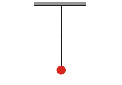
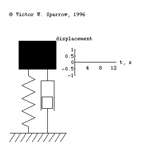
As seen from above, both the cases represent a sinusoidal characterstic and where in the case of pendulum, the damping force is the declining rate of conversion of Potential Energy to Kinetic Energy, in the Spring-Mass-Damper system it is the conversion of Kinetic Energy to Heat Energy.

The system taken for this report will be provided an initial perturbance of 3[rad/s] at time t=0 and the value of angular displacement on the first step would be 0.

Code:

(1) Auxiliary Code(Function): This is the function code within which, our mathematical equations will be stored and through this function itself, these will be executed.

function [dtheta_dt]=ode_func(t,tht,b,g,l,m)
tht1=tht(1);
tht2=tht(2);
dtheta1_dt=tht2;
dtheta2_dt=-(b/m)*tht2-(g/l)*sin(tht1);
dtheta_dt=[dtheta1_dt; dtheta2_dt];
end

As seen in the code lines four and five, the function script uses the equations (i) and (ii) of our mathematical procedure and outputs the results into the vector called 'dtheta_dt'.

The function takes inputs for time(t), angle(theta), damping factor(b), gravitational acceleration(g), length of string(l) and mass of the bob(m) where theta is the vector to the LHS which contains the values of `theta_1`(displacement) and `theta_2`(velocity).

(2) Main Code: In order to bring all the variables together, and produce a time, displacement and a velocity vector, the main code employs our function and is also responsible for generating the movie file.

2.1 System Inputs:

2.1.1 Damping factor(b)

b=0.05;

2.1.2 Gravitational Acceleration(g [m/s^2])

g=9.81;

2.1.3 Length of string(l [m])

l=1;

2.1.4 Mass of the bob(m [kg])

m=1;

2.1.5 Initial Conditions: Displacement & Velocity (`theta_1` & `theta_2`)

tht_0=[0;3];

2.1.6 Time Scale

t_span=linspace(0,20,300);

2.2 Calling the function and solving the ODE:

[t, results]=ode45(@(t,tht) ode_func(t,tht,b,g,l,m),t_span,tht_0);
figure(1)
plot(t,results)
hold on
plot(t,results)
ylabel('Velocity and Displacement')
xlabel('Time')
tht=results(:,1);
ct=1;
for i=1:length(tht)
    THT=tht(i);
    figure(2)
    x0=0;
    y0=0;
    x1=l*cos(3*pi/2+THT);
    y1=l*sin(3*pi/2+THT);
    plot([x0 x1],[y0 y1],'k','Linewi',2)
    hold on
    plot(x1,y1,'m.','markers',40)
    plot([-3, 3],[0,0],'k','Linewi',6)
    hold off
    axis([-3,3,-2,2])
    pause(0.05)
    M(ct)=getframe(gcf);
    ct=ct+1;
end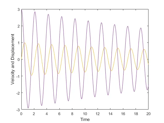

• The solver used for this code is ODE45 which is called in relation to the outputs presented by the function 'ode_func' which are t and tht and the results from each is then saved into 't' and 'results' respectively where results is a N*2 matrix and t is a N*1 vector.
• Here 'i' is the index variable which is responsible for keeping track of the displacement values stored in the first column of 'results'.
• Here, 'ct' is the loop counter that is responsible to index all the snapshots generated by running the loop through time and would be used to generate the movie file.
• The co-ordinates x1 and y1 are taken as sin of added values over (3*pi/2) so as to rotate the figure by 270-degrees, counter-clockwise.
• 'axis' command is responsible for properly scaling the simulation result.

2.3 Error Description: In the initial stages, the script displayed undesired result in which the orentation of the pendulum itself was incorrect as seen from the picture below:

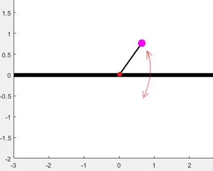
Here, the plane seems to be rotated around by negative-270-degrees and could be corrected if 3*pi/2 is added to the instantaneous angle 'THT' at every time step.

Another potential source of error could be seen while generating the movie as the following lines of code are case-sensitive.

2.4 Generting the Movie:

movie(M)
videofile=VideoWriter('pendulumvideo.avi','uncompressed AVI');
open(videofile)
writeVideo(videofile,M)
close(videofile)

2.3.1 Movie Link(YouTube): Motion of a simple pendulum

Conclusion:

• From the video, it is evident that with a small damping factor and a large mass, it becomes really difficult for the bob to come to rest within the 20-second time window.
• From the output plot, the state of damping in this system is apparent which is a gradual decline.
• The same skeleton could be used to solve a seperate 2nd-order ODE for another application in the future.