Project 2 - Rankine cycle Simulator

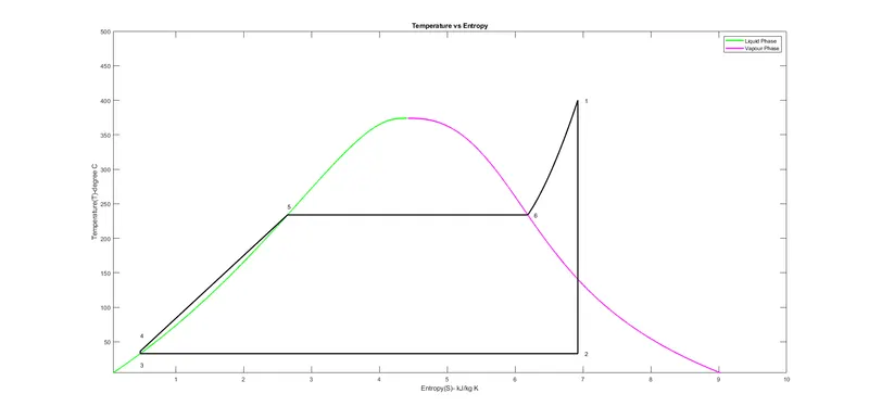
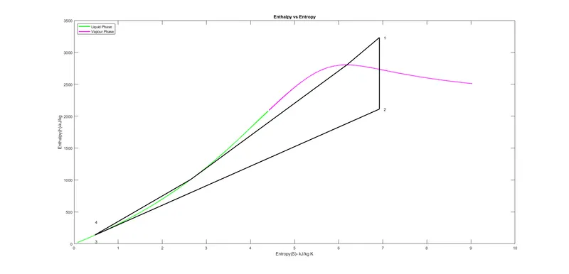
1. Aim: To build a simulator which displays results based on the XSteam Library and displays the Rankine Cycle T-S and H-S Curves. Along with this, our script must also display some results on to the command window with a complete simulator-like environment.

2. Object Description:

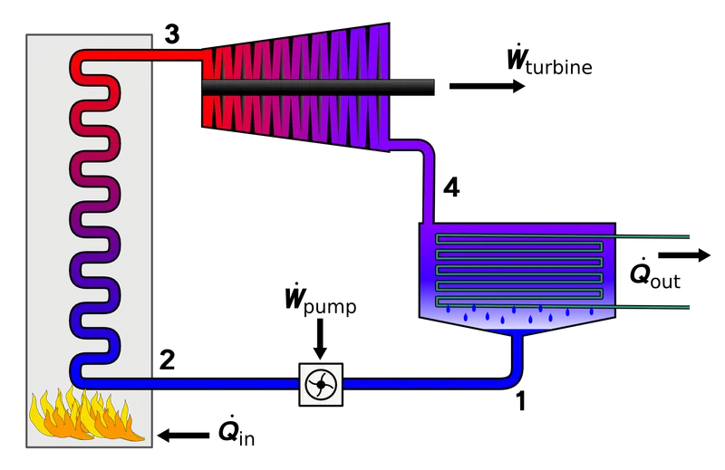
2.1 Rankine Cycle: The Rankine Cycle is an idealized thermodynamic cycle which demonstrates the process by which certain heat engines like steam turbines or reciprocating steam engines allows the mechanical work to be extracted from a fluid as it moves between the heat source and the heat sink within a system.

This is an external combustion process as the heat energy is supplied to the system via a Boiler where the working fluid(typically water) is converted to a high-pressure steam which then moves further through the system turing the turbine. After passing through the turbine, the fluid is converted back to liquid state by means of condensation and the heat energy is rejected as wastage from the system before this fluid again returns to the boiler, completing one cycle.

Note: Friction losses throughout the system are often neglected for the purpose of simplifying calculations as such losses are usually much less significant than thermodynamic losses, especially in larger systems.

Methods to increase efficiency of the rankine cycle:

1. Lowering Condenser pressure: Lowering the operating pressure of the condenser lowers the temperature at which heat is rejected. The overall effect of lowering the condenser pressure is an increase in the thermal efficiency of the cycle.
2. Superheating the steam to high temperatures: The average temperature at which heat is added to the steam can be increased without increasing the boiler pressure by superheating the steam to high temperatures. Superheating the steam also decreases the moisture content of the steam at the turbine exit.
3. Increasing boiler pressure: Increasing the operating pressure of the boiler, automatically raises the temperature at which boiling takes place. This raises the average temperature at which heat is added to the steam and thus raises the thermal efficiency of the cycle.

Given below is the system layout for the Rankine Cycle:

2.2 Rankine Cycle Simulator: This is a Matlab script where the results are based on three main user inputs- The turbine inlet pressure and temperature and turbine outlet pressure. Apart from this, the XSteam library forms the fundamental structure for this script to output the desired results.

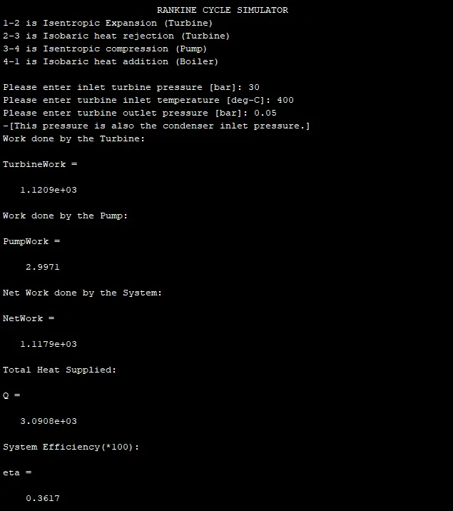
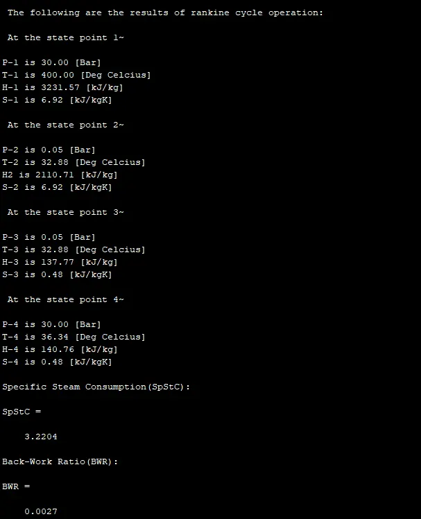
The output to expect in the command window from this script includes:

• Process description.
• Work done by Turbine and Pump individually.
• Net work done by the system.
• Total heat provided to the system.
• System overall efficiency.
• Values for Temperature, Pressure, Entropy and Enthalpy at the four state points.
• Specific Steam Consumption.
• Lastly, the Back-work ratio.

Along with these, the script also outputs two figures: the T-S Diagram and the H-S diagram.

3. Code:

3.1 Main Script-

Rankine Cycle Simulator based on the XSteam library

fprintf('%50s','RANKINE CYCLE SIMULATOR')
disp(' ')
fprintf('1-2 is Isentropic Expansion (Turbine) \n')
fprintf('2-3 is Isobaric heat rejection (Turbine) \n')
fprintf('3-4 is Isentropic compression (Pump) \n')
fprintf('4-1 is Isobaric heat addition (Boiler) \n')
disp(' ')

Taking user input:

% Message 1
x=input('Please enter inlet turbine pressure [bar]: ');
p1=x;
% Message 2
y=input('Please enter turbine inlet temperature [deg-C]: ');
t1=y;
% Message 3
z=input('Please enter turbine outlet pressure [bar]: ');
p2=z;
fprintf('-[This pressure is also the condenser inlet pressure.] \n')

Parameters for Turbine Inlet (State Point-1):

tsat=XSteam('Tsat_p',p1);
h1=XSteam('h_pT',p1,t1);
s1=XSteam('s_pT',p1,t1);

Parameters for Turbine Outlet (State Point-2):

s2=s1; % Isentropic Process
sf2=XSteam('sL_p',p2);
sg2=XSteam('sv_p',p2);

Dryness Fraction:

x2=(s2-sf2)/(sg2-sf2);
t2=XSteam('T_ps',p2,s2);
h2=XSteam('h_px',p2,x2);
hf2=XSteam('hL_p',p2);

Parameters for Pump Inlet (State Point-3):

p3=p2;
t3=t2;
s3=sf2;
h3=hf2;
t5=tsat;

Parameters for boiler inlet (State Point-4):

s4=s3;
p4=p1;
h4=XSteam('h_ps',p4,s4);
cp=XSteam('cp_ps',p4,s4);
cv=XSteam('cv_ps',p4,s4);
c=cp/cv;
t4=t3*((p4/p3)^(c-1)/c);

Parameters for Points 5 & 6:

h5=XSteam('hL_p',p1);
s5=XSteam('sL_p',p1);
t6=t1;
h6=XSteam('hV_p',p1);
s6=XSteam('sV_p',p1);

Computation of important results:

% 1) Work done by the turbine
disp('Work done by the Turbine:')
TurbineWork=h1-h2

% 2) Work done by the pump
disp('Work done by the Pump:')
PumpWork=h4-h3

% 3) Net work done
disp('Net Work done by the System:')
NetWork=TurbineWork-PumpWork

% Supplied heat and overall efficiency
disp('Total Heat Supplied:')
Q=h1-h4
disp('System Efficiency(*100):')
eta=NetWork/Q

T-S Diagram:

T=linspace(5,400,25000);
for i=1:length(T)
    s(i)=XSteam('sL_t',T(i));
    S(i)=XSteam('SV_t',T(i));
    h(i)=XSteam('hL_t',T(i));
    H(i)=XSteam('hV_t',T(i));
end
figure(1)
plot(s,T,'g','linewi',2)
hold on 
plot(S,T,'m','linewi',2)
plot([s1 s2 s3 s4 s5 s6],[t1 t2 t3 t4 t5 tsat],'k',...
    'linewi',2)
title('Temperature vs Entropy')
axis([1,10,10,500])
ylabel('Temperature [C]')
xlabel('Entropy [KJ/Kg-K]')
text(s1+0.1, t1, '1')
text(s2+0.1, t2, '2')
text(s3, t3-16, '3')
text(s4, t4+23, '4')
text(s5,t4+210,'5')
text(s6+0.09,t5,'6')

Saturated Temperature (curve joining Pt. 6 to Pt. 1):

k=linspace(tsat,t1,500);
for i=1:length(k)
    d(i)=XSteam('s_pT',p1,k(i));
end
plot(d,k,'linewidth',2,'color','k')
title('Temperature vs Entropy')
xlabel('Entropy(S)- kJ/kg K')
ylabel('Temperature(T)-degree C')
legend('Liquid Phase','Vapour Phase')

H-S Curve:

figure(2)
plot(s,h,'g','linewi',2);
hold on
plot(S,H,'m','linewi',2);
plot([s1 s2],[h1 h2],'k','linewi',2)
plot([s2 s3],[h2 h3],'k','linewi',2)
plot([s3 s4],[h3 h4],'k','linewi',2)
plot([s4 s5],[h4 h5],'k','linewi',2)
plot([s5 s6],[h5 h6],'k','linewi',2)
plot([s6 s1],[h6 h1],'k','linewi',2)
text(s1+0.1, h1, '1')
text(s2+0.1, h2, '2')
text(s3, h3-100, '3')
text(s4, h4 +200, '4')
title('Enthalpy vs Entropy')
xlabel('Entropy(S)- kJ/kg K')
ylabel('Enthalpy(h)-kJ/kg')
legend('Liquid Phase','Vapour Phase','location','northwest')

Printing to the Command Window:

disp(' The following are the results of rankine cycle operation: ')
disp(' ')
disp(' At the state point 1~')
disp(' ')
n1=sprintf('P-1 is %.2f [Bar]',p1);
disp(n1)
n2=sprintf('T-1 is %.2f [Deg Celcius]',t1);
disp(n2)
n3=sprintf('H-1 is %.2f [kJ/kg]',h1);
disp(n3)
n4=sprintf('S-1 is %.2f [kJ/kgK]',s1);
disp(n4)

disp(' ')
disp(' At the state point 2~')
disp(' ')
n5=sprintf('P-2 is %.2f [Bar]',p2);
disp(n5)
n6=sprintf('T-2 is %.2f [Deg Celcius]',t2);
disp(n6)
n7=sprintf('H2 is %.2f [kJ/kg]',h2);
disp(n7)
n8=sprintf('S-2 is %.2f [kJ/kgK]',s2);
disp(n8)

disp(' ')
disp(' At the state point 3~')
disp(' ')
n9=sprintf('P-3 is %.2f [Bar]',p3);
disp(n9)
n10=sprintf('T-3 is %.2f [Deg Celcius]',t3);
disp(n10)
n11=sprintf('H-3 is %.2f [kJ/kg]',h3);
disp(n11)
n12=sprintf('S-3 is %.2f [kJ/kgK]',s3);
disp(n12) 

disp(' ')
disp(' At the state point 4~')
disp(' ')
n13=sprintf('P-4 is %.2f [Bar]',p4);
disp(n13)
n14=sprintf('T-4 is %.2f [Deg Celcius]',t4);
disp(n14)
n15=sprintf('H-4 is %.2f [kJ/kg]',h4);
disp(n15)
n16=sprintf('S-4 is %.2f [kJ/kgK]',s4);
disp(n16)
disp(' ')

Specific Steam Consumption:

disp('Specific Steam Consumption(SpStC):')
SpStC=3600/NetWork

Back Work Ratio: The fraction of work done by Turbine that is consumed by the Pump.

disp('Back-Work Ratio(BWR):')
BWR=PumpWork/TurbineWork

4. Results:

4.1 T-S Diagram:

4.2 H-S Diagram:

4.3 Command Window Output:

5. Sources:

1. Rankine Cycle Wikipedia.
2. Ideal Rankine Cycle.
3. Rankine Cycle YT.