Drive Cycle Programming for Vechiles
Aim : To create and plot Matlab codes for different Drive Cycle Plots
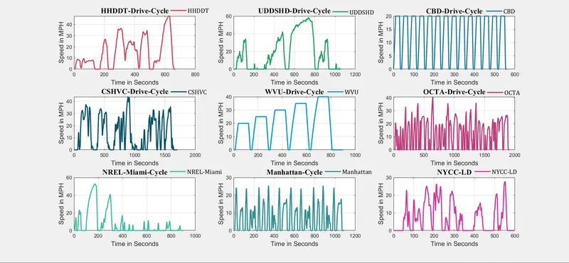
Objective : To create and plot Matlab codes for Nine different Drive Cycles in a 3 x 3 Matrix.
Introduction :
- A drive cycle is typically represented by a series of data points which plots vechile speed against time.
- Driving cycles are produced to assess the performance of vehicles in various ways i.e fuel consumption and pollutant emissions.
Programming Part
clear;
clc;
close all;
%% Drive-Cycle-1
figure(1);
subplot(3,3,1);
drivecycle1= readtable("HHDDT.csv");
x=drivecycle1.Time_seconds_;
y= drivecycle1.Speed_mph_;
plot(x,y,'color','#d9445f',"LineWidth",2);
title("HHDDT-Drive-Cycle","FontSize",14,"FontName","Times New Roman");
xlabel("Time in Seconds","FontSize",12,"FontName","SansSerif");
ylabel("Speed in MPH","FontSize",12,"FontName","SansSerif");
legend("HHDDT","FontSize",12,"FontName","Cambria");
legend("boxoff");
grid on;
%% Drive-Cycle-2
figure(1);
subplot(3,3,2);
drivecycle2= readtable("UDDS_HD.csv");
x=drivecycle2.Time_seconds_;
y=drivecycle2.Speed_mph_;
plot(x,y,'Color','#22a364',"LineWidth",2);
title("UDDSHD-Drive-Cycle","FontSize",14,"FontName","Times New Roman");
xlabel("Time in Seconds","FontSize",12,"FontName","SansSerif");
ylabel("Speed in MPH","FontSize",12,"FontName","SansSerif");
legend("UDDSHD","FontSize",12,"FontName","Cambria");
legend("boxoff");
grid on;
%% Drive-Cycle-3
figure(1);
subplot(3,3,3);
drivecycle3= readtable("CBD.csv");
x=drivecycle3.Time_seconds_;
y=drivecycle3.Speed_mph_;
plot(x,y,'Color','#227ca3',"LineWidth",2);
title("CBD-Drive-Cycle","FontSize",14,"FontName","Times New Roman");
xlabel("Time in Seconds","FontSize",12,"FontName","SansSerif");
ylabel("Speed in MPH","FontSize",12,"FontName","SansSerif");
legend("CBD","FontSize",12,"FontName","Cambria");
legend("boxoff");
grid on;
%% Drive-Cycle-4
figure(1);
subplot(3,3,4);
drivecycle4= readtable("CSHVC.csv");
x=drivecycle4.Time_seconds_;
y=drivecycle4.Speed_mph_;
plot(x,y,'Color','#065065',"LineWidth",2);
title("CSHVC-Drive-Cycle","FontSize",14,"FontName","Times New Roman");
xlabel("Time in Seconds","FontSize",12,"FontName","SansSerif");
ylabel("Speed in MPH","FontSize",12,"FontName","SansSerif");
legend("CSHVC","FontSize",12,"FontName","Cambria");
legend("boxoff");
grid on;
%% Drive-Cycle-5
figure(1);
subplot(3,3,5);
drivecycle5= readtable("WVU.csv");
x=drivecycle5.Time_seconds_;
y=drivecycle5.Speed_mph_;
plot(x,y,'Color','#069ac3',"LineWidth",2);
title("WVU-Drive-Cycle","FontSize",14,"FontName","Times New Roman");
xlabel("Time in Seconds","FontSize",12,"FontName","SansSerif");
ylabel("Speed in MPH","FontSize",12,"FontName","SansSerif");
legend("WVU","FontSize",12,"FontName","Cambria");
legend("boxoff");
grid on;
%% Drive-Cycle-6
figure(1);
subplot(3,3,6);
drivecycle6= readtable("OCTA.csv");
x=drivecycle6.Time_seconds_;
y=drivecycle6.Speed_mph_;
plot(x,y,'Color','#be3d7c',"LineWidth",2);
title("OCTA-Drive-Cycle","FontSize",14,"FontName","Times New Roman");
xlabel("Time in Seconds","FontSize",12,"FontName","SansSerif");
ylabel("Speed in MPH","FontSize",12,"FontName","SansSerif");
legend("OCTA","FontSize",12,"FontName","Cambria");
legend("boxoff");
grid on;
%% Drive-Cycle-7
figure(1);
subplot(3,3,7);
drivecycle7= readtable("NREL-Miami.csv");
x=drivecycle7.Time_seconds_;
y=drivecycle7.Speed_mph_;
plot(x,y,'Color','#3dbea1',"LineWidth",2);
title("NREL-Miami-Cycle","FontSize",14,"FontName","Times New Roman");
xlabel("Time in Seconds","FontSize",12,"FontName","SansSerif");
ylabel("Speed in MPH","FontSize",12,"FontName","SansSerif");
legend("NREL-Miami","FontSize",12,"FontName","Cambria");
legend("boxoff");
grid on;
%% Drive-Cycle-8
figure(1);
subplot(3,3,8);
drivecycle8= readtable("Manhattan.csv");
x=drivecycle8.Time_seconds_;
y=drivecycle8.Speed_mph_;
plot(x,y,'Color','#308f93',"LineWidth",2);
title("Manhattan-Cycle","FontSize",14,"FontName","Times New Roman");
xlabel("Time in Seconds","FontSize",12,"FontName","SansSerif");
ylabel("Speed in MPH","FontSize",12,"FontName","SansSerif");
legend("Manhattan","FontSize",12,"FontName","Cambria");
legend("boxoff");
grid on;
%% Drive-Cycle-9
figure(1);
subplot(3,3,9);
drivecycle9= readtable("NYCC-LD.csv");
x=drivecycle9.Time_seconds_;
y=drivecycle9.Speed_mph_;
plot(x,y,'Color','#d6369a',"LineWidth",2);
title("NYCC-LD","FontSize",14,"FontName","Times New Roman");
xlabel("Time in Seconds","FontSize",12,"FontName","SansSerif");
ylabel("Speed in MPH","FontSize",12,"FontName","SansSerif");
legend("NYCC-LD","FontSize",12,"FontName","Cambria");
legend("boxoff");
grid on;
Output Plots