Discretization for range of dx

Aim : To compute the first, second and fourth order approximations for a range of dx

Here we have modified the previous code by adding a for loop and taking the range for dx

% A program that compares the first, second and fourth order approximations
% of the first derivative against the analytical or exact derivative

clc % clears the command window
clear % clears the workspace
close all % closes all the windows opened by matlab

% values at which function needed to be found
x=pi/3; 
d_x=linspace(pi/4000,pi/40,20);

% Main function
f_x=sin(x)/x^3; 
for i=1:length(d_x)
  dx=d_x(i);  
% Taylor variables f(x+dx),f(x-dx),f(x+2dx),f(x-2dx)
f_xplusdx=sin(x+dx)/(x+dx)^3;
f_xminusdx=sin(x-dx)/(x-dx)^3;
f_xplus2dx=sin(x+2*dx)/(x+2*dx)^3;
f_xminus2dx=sin(x-2*dx)/(x-2*dx)^3;

% Analytically or exact derivative
fdash_x=cos(x)/x^3-3*sin(x)/x^4;

% Numerically 

% first, order approximations of the first derivative
forward_diff=(f_xplusdx-f_x)/dx; 
error1(i)=abs(forward_diff-fdash_x);

% second order approximations of the first derivative
central_diff=(f_xplusdx-f_xminusdx)/(2*dx);
error2(i)=abs(central_diff-fdash_x);

% fourth order approximations of the first derivative
fourth_order=(f_xminus2dx-8*f_xminusdx+8*f_xplusdx-f_xplus2dx)/(12*dx);
error4(i)=abs(fourth_order-fdash_x);



end

figure (1)
loglog(d_x,error1,'color','red')
hold on
loglog(d_x,error2,'color','green')
loglog(d_x,error4,'color','blue')
xlabel('d_x') % Labelling X-axis
ylabel('ERROR') % Labelling Y-axis
legend('First','Second','Fourth') % Legend


figure (2)
plot(log(d_x),log(error1),'color','red')
hold on
plot(log(d_x),log(error2),'color','green')
plot(log(d_x),log(error4),'color','blue')
xlabel('d_x') % Labelling X-axis
ylabel('ERROR') % Labelling Y-axis
legend('First','Second','Fourth') % Legend

OUTPUT:

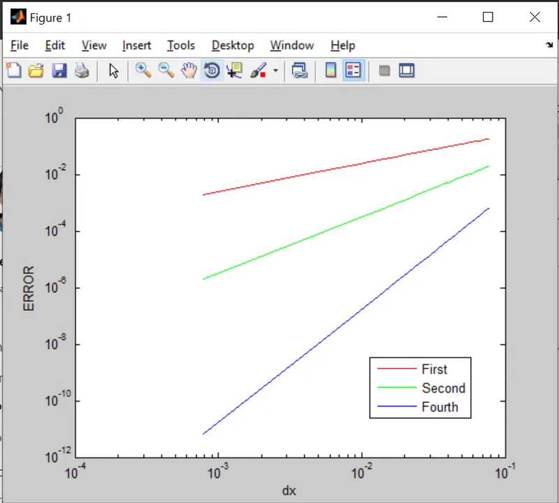
Here, we have plotted output in loglog form because this graph makes sense as the previous graph values are abrupt

So, to calculate the slope of the graph the values should also be in log so I have plotted another graph with log values below

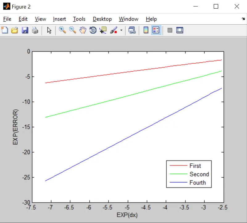
So, now lets calculate slope

(1) For 1st order approximation

- m=(y2-y1)/(x2-x1) = (-1.7226 - -6.23328)/(-2.544147 - -7.14931)= 0.97948

(2) For 2nd order approximation

- m=(y2-y1)/(x2-x1) = (-3.9240 - -13.14256)/(-2.544147 - -7.14931)= 2.001765

(4) For 4th order approximation

- m=(y2-y1)/(x2-x1) = (-7.283467 - -25.734)/(-2.544147 - -7.14931)= 4.006482

As we can see that the slope of the 4th order approximation curve is higher than second and first therefore

It will lead to accurate solution 4 times faster while 2nd order 2 times faster than first order.