Cyclone Separator Challenge
Aim:- To perform analysis on cyclone separator and calculate the separation efficiency and pressure drop.
Objective:-
- To write a few words about any four empirical models used to calculate the cyclone separator efficiency.
- To perform an analysis on a given cyclone separator model by varying the particle diameter from 1 μm to 5 μm and calculate the separation efficiency in each case. Discuss the results. [Use both the velocity's as 3m/sec].
- To perform an analysis on a given cyclone separator model by varying the particle velocity from 1 m/sec to 5 m/sec and calculate the separation efficiency and pressure drop in each case. Discuss the results. [Use particle diameter size as 5 μm for all cases & keep flow velocity same as particle velocity].
Given conditions:
Inlet and wall:- Reflect.
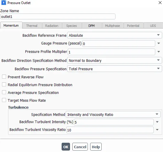
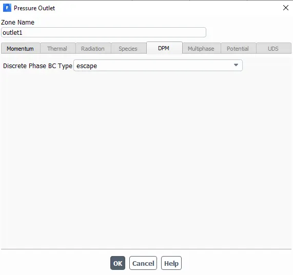
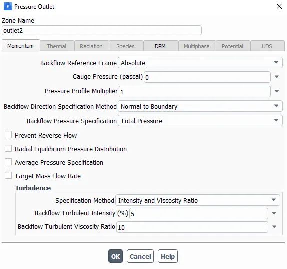
Outlet(Top):- Escape.
Outlet(Bottom/dustbin) - Trap.
Cyclone Separator:
Cyclone separators or simply cyclones are separation devices (dry scrubbers) that use the principle of inertia to remove particulate matter from flue gases. Cyclone separators are one of many air pollution control devices known as pre-cleaners since they generally remove larger pieces of particulate matter.
Cyclone separation is a method of removing particulates from an air, gas, or liquid stream, without the use of filters, through vortex separation. When removing particulate matter from liquid, a hydro-cyclone is used; while from gas, a gas cyclone is used.
This prevents finer filtration methods from having to deal with large, more abrasive particles later on. In addition, several cyclone separators can operate in parallel, and this system is known as a multi-cyclone.
It is important to note that cyclones can vary drastically in their size. The size of the cyclone depends largely on how much flue gas must be filtered, thus larger operations tend to need larger cyclones.
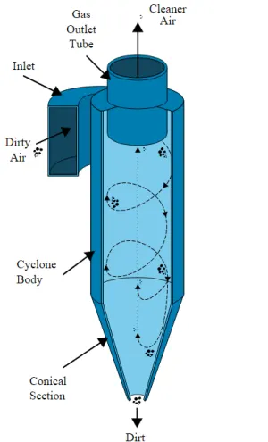
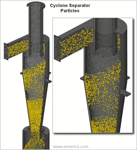
Cyclone separators work much like a Centrifuge, but with a continuous feed of dirty air. In a cyclone separator, dirty flue gas is fed into a chamber. The inside of the chamber creates a spiral vortex, similar to a tornado. This spiral formation and the separation is shown in Figure. The lighter components of this gas have less inertia, so it is easier for them to be influenced by the vortex and travel up it. Contrarily, larger components of particulate matter have more inertia and are not as easily influenced by the vortex.
Since these larger particles have difficulty following the high-speed spiral motion of the gas and the vortex, the particles hit the inside walls of the container and drop down into a collection hopper. These chambers are shaped like an upside-down cone to promote the collection of these particles at the bottom of the container. The cleaned flue gas escapes out the top of the chamber.
Most cyclones are built to control and remove particulate matter that is larger than 10 micrometers in diameter. However, there do exist high-efficiency cyclones that are designed to be effective on particles as small as 2.5 micrometers. As well, these separators are not effective on extremely large particulate matter. For particulates around 200 micrometers in size, gravity settling chambers or momentum separators are a better option.
Out of all of the particulate-control devices, cyclone separators are among the least expensive. They are often used as a pre-treatment before the flue gas enters more effective pollution control devices. Therefore, cyclone separators can be seen as "rough separators" before the flue gas reaches the fine filtration stages.
Types of empirical models used to calculate the cyclone separator efficiency:
Iozia and Leith model :
Iozia and Leith (1990) logistic model is a modified version of Barth (1956) model which is developed based on force balance. The model assumes that a particle carried by the vortex endures the influence of two forces: a centrifugal force, Z, and flow resistance,
The addition made by Iozia and Leith on the original Barth (1956) model is the core length zc and slope parameter β expression which is derived based on the statistical analysis of experimental data of cyclone with D = 0.25 m.
LI and Wang Model:
The Li and Wang (1989) model include particle bounce or re-entrainment and turbulent diffusion at the cyclone wall. A two-dimensional analytical expression of particle distribution in the cyclone is obtained. Li and Wang model was developed based on the following assumptions:
- The radial particle velocity and the radial concentration profile are not constant, for uncollected particles within the cyclones.
- Boundary conditions with the consideration of turbulent diffusion coefficient and particle bounce re-entrainment on the cyclone wall
Koch and Licht Model:
Koch and Licht (1977) collection theory recognized the inherently turbulent nature of cyclones and the distribution of gas residence times within the cyclone. Koch and Licht describe particle motion in the entry and collection regions with the additional following assumptions:
- The tangential velocity of a particle is equal to the tangential velocity of the gas flow, i.e. there is no slip in the tangential direction between the particle and the gas.
- The tangential velocity is related to the radius of cyclone by uRn = constant.
Lapple Model:
Lapple (1951) model was developed based on force balance without considering the flow resistance. Lapple assumed that a particle entering the cyclone is evenly distributed across the inlet opening. The particle that travels from inlet half-width to the wall in the cyclone is collected with 50% efficiency. The semi-empirical relationship developed by Lapple (1951) to calculate a 50% cut diameter.
Applications:
- Chemical and Petrochemical Processes.
- Industrial, Metallurgical, and Power Generation.
- Food & Pharmaceutical.
- Cement Industry.
Methodology:
There are two different Phases as given below:
- Continuous Phase
- Discrete Phase
continuous Phase:
- It consists of fluid flowing within the fluid volume.
Discrete Phase:
- It consists of smaller particles interacting with the continuous phase.
- It can also exchange momentum, mass, and energy with Fluid Phase or Continuous Phase.
To carry out this analysis,
- The simulation will be done using DPM (Discrete Phase Modeling).
Discrete Phase Modeling:
- It is employed when there are solid Particles in Gas, or Liquid or Liquid Droplets in Gas, or Bubbles in Liquid.
There are two ways to carry out DPM
- Un-coupled Flow
- Coupled Flow
Uncoupled Flow:
In this type of flow, the Discrete Phase will not have any interaction with the Continuous Phase.
Coupled Flow:
- It will influence the flow of the Continuous Phase.
Since the size of the particles injected into the CycloneSeparator is very small, the usage of both types of flow should not matter much.
Simulation Procedure:
Geometry:
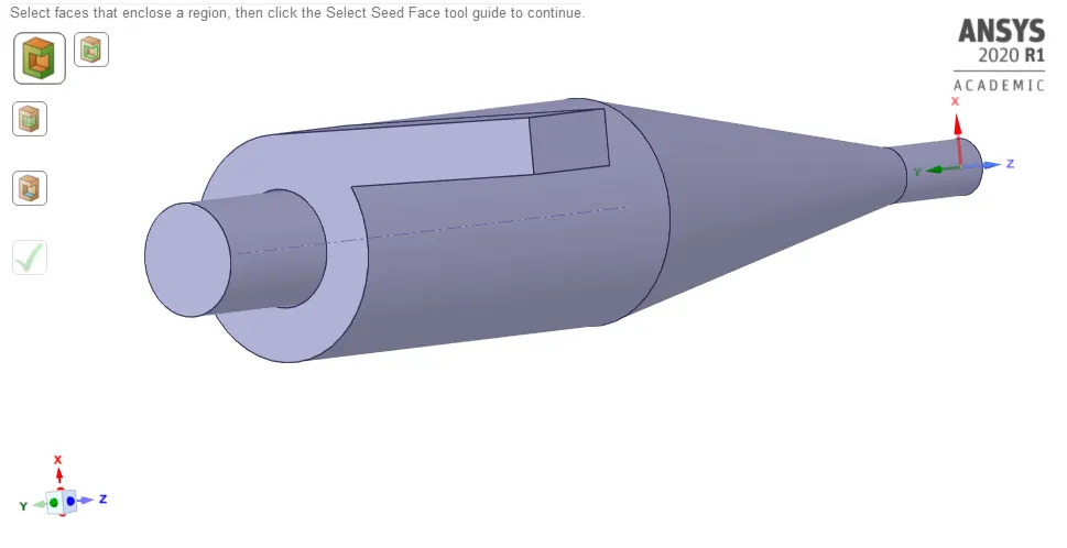
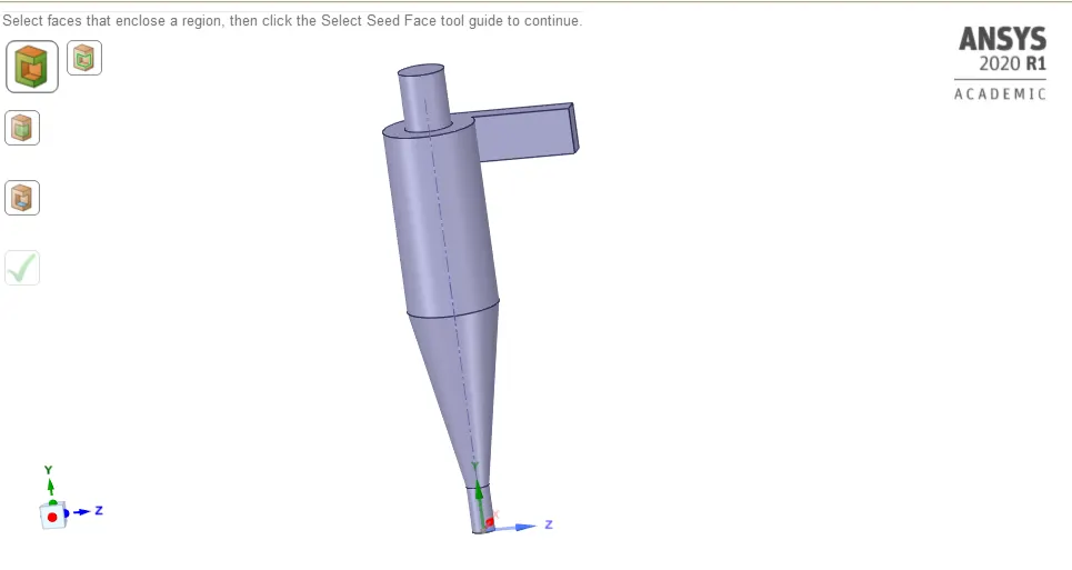
Given Geometry:
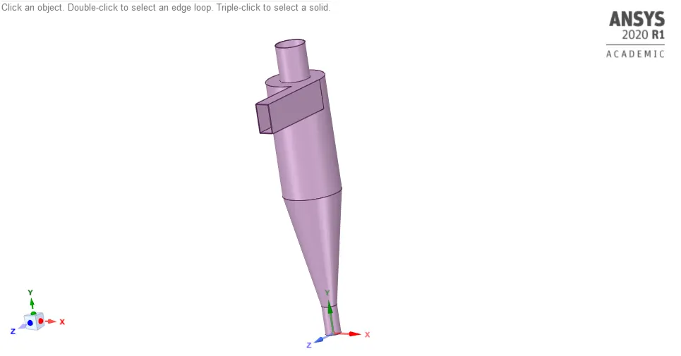
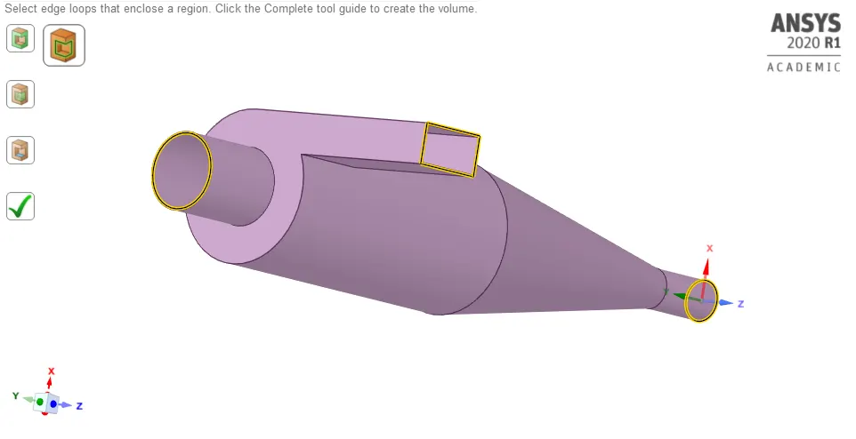
Volume Extract:
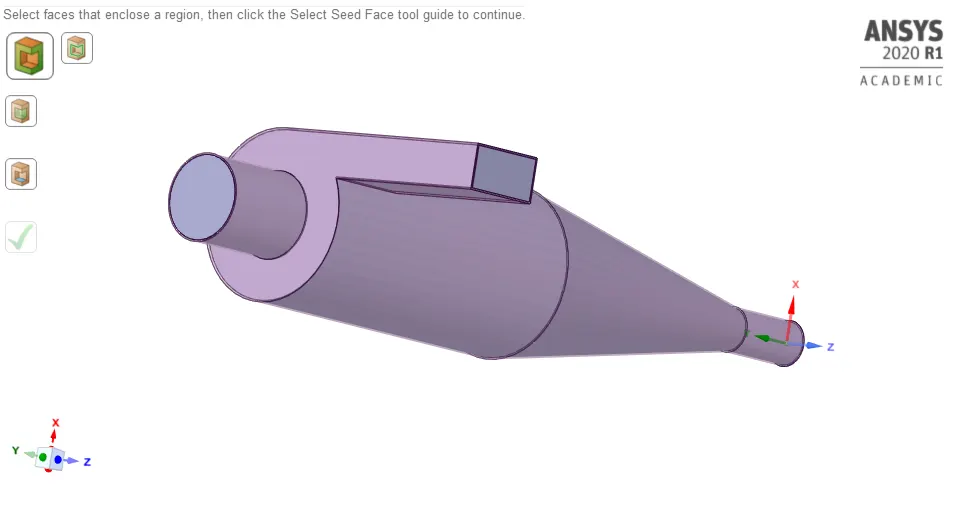
Suppress for physics and unselect it:
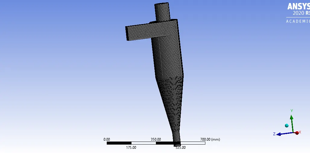
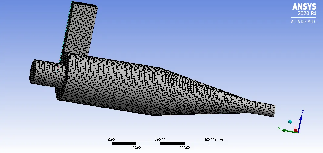
Meshing:
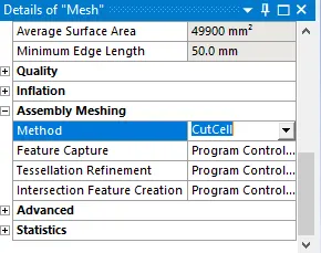
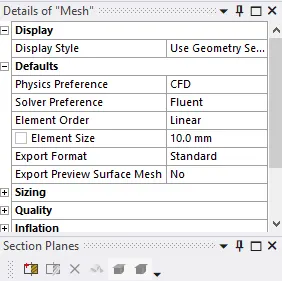
For better results, we used cutcell meshing approach available in Ansys Meshing.
Mesh:
Mesh Sizing:
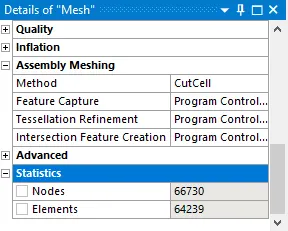
Statistics:
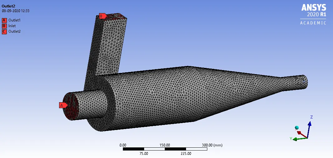
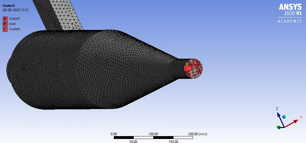
Named Selections:
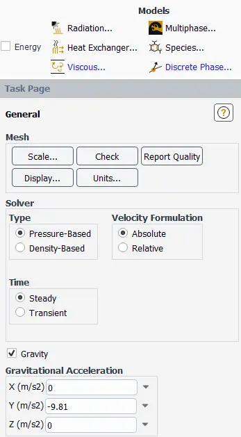
SetUp:
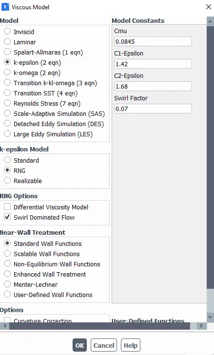
Here RNG is the slight modification of the standard K-Epsilon model. This enhances the accuracy of the swirling flows.
DPM Settings:
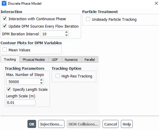
As per the above image, enable the “Interaction with Continuous Phase”. This will enable the Coupled Flow.
Also, enable “Update DPM Sources Every Flow Iteration”. Enabling this option gives the chance to calculate the Particle Source Terms at every Iteration. (For Unsteady Simulation, it is recommended, and given by-default.)
Set “DPM Iteration Interval = 10”. This option allows us to control the frequency at which particles attract.
Here “Tracking Parameters =50000”. It is the maximum number of Time Steps, to compute a single trajectory of Particle. In case, the fluent exceeds the maximum number of Time Steps, it will automatically cancel the report of Trajectory. For the Steady case, Time Steps number = 50,000 given by default. But for calculation of all possible particles, we have set it to be the same as 50000.
Length scale=5m.Here, we have used the “Specify Length Scale”, which is used for controlling the Time Step size, by dividing Length Scale with Velocity of Discrete Particle and Velocity with Velocity of Continuous Phase.
The length scale is also used to control the size of the Time Step. The larger the Factor, the smaller the Time Step will be.
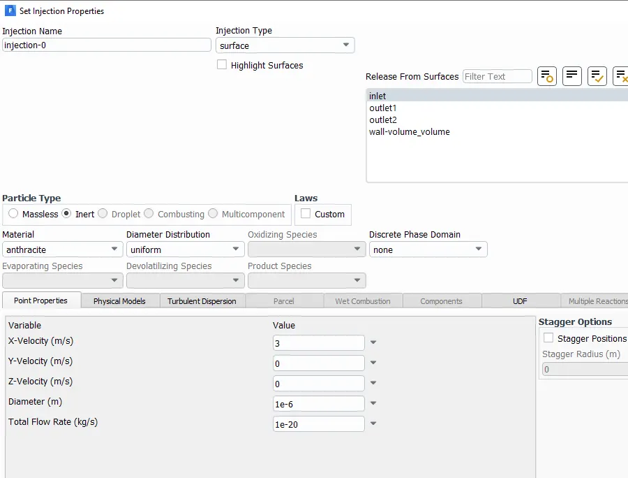
Injections:
Boundary conditions:
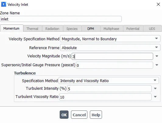
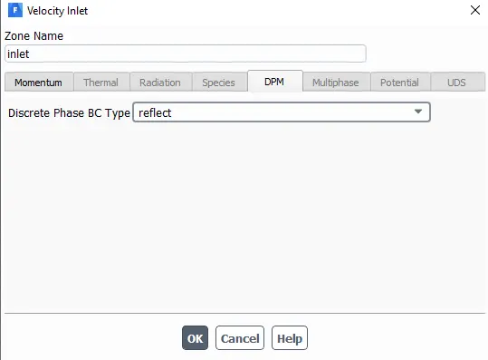
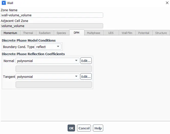
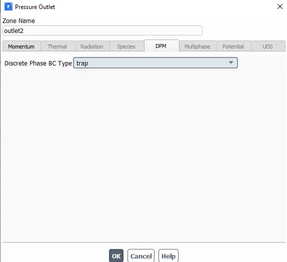
Reflect: It is the Particle Rebound off the boundary in question with a change in its momentum as defined by the coefficient of restitution.
Escape: The particle is reported as having “escaped” when it encounters the boundary in question. Trajectories calculated are terminated.
Trap: The Trajectory calculated is terminated and the fate of the particle is recorded as “trapped”. In the case of evaporating droplets, their entire mass instantaneously passes into the vapor phase and enters the Cell adjacent to the boundary. IN the case of a combusting particle, the remaining volatile mass is passed into the vapor phase.
Solutions Methods:
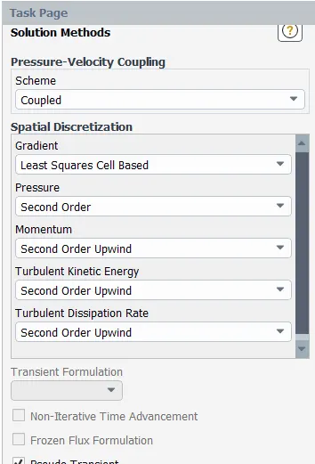
-
Apart from all default settings, we have changed some of the settings as suggested in the above image, for this type of analysis.
Here, we have set Momentum of “Turbulent Kinetic Energy” & “Turbulent Dissipation Rate” to the Second-Order Upwind scheme.
This type of analysis can give us more accurate results.
Initialization:
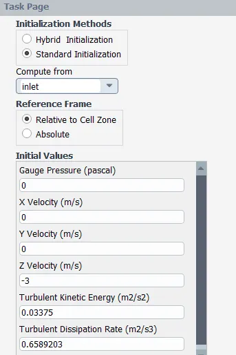
Here, as per the above image, we have set the “Standard initialization”. Also, the computing option has been set to “Compute From = Inlet”.
If we have Inlets and Outlets, then we can go for Standard Initialization, and it is best suited for this type of Analysis.
Run Calculation:
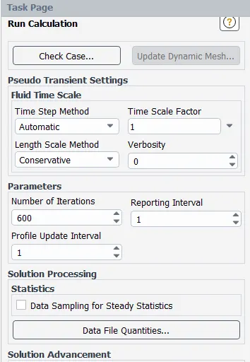
Results:
Case1:
Inlet velocity=3m/sec.
varying the particle diameter from 1 μm to 5 μm.
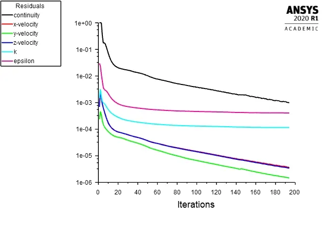
(A). Particle Diameter=1 μm
Residual Plots:
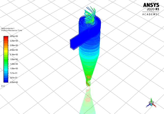
Particle Residence Time:
Particle Tracking:

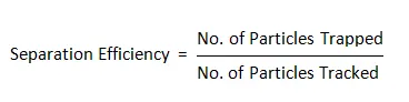
Separation Efficiency in % = (25 / 98) * 100
Separation Efficiency = 25.5 %
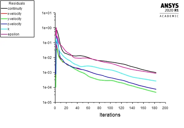
(B). Particle Diameter=2 μm
Residual Plots:
Particle Residence Time:
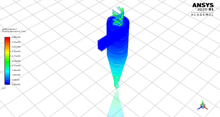
Particle Tracking:

Separation Efficiency in % = (59 / 98) * 100
Separation Efficiency = 60.20 %
(C). Particle Diameter=3 μm
Residual Plots:
Particle Residence Time:
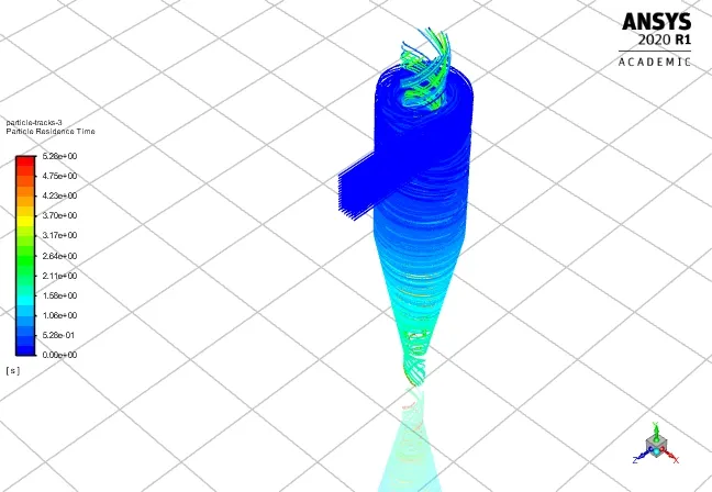
Particle Tracking:

Separation Efficiency in % = (63 / 98) * 100
Separation Efficiency = 64.2 %
(D). Particle Diameter=4 μm
Residual Plots:
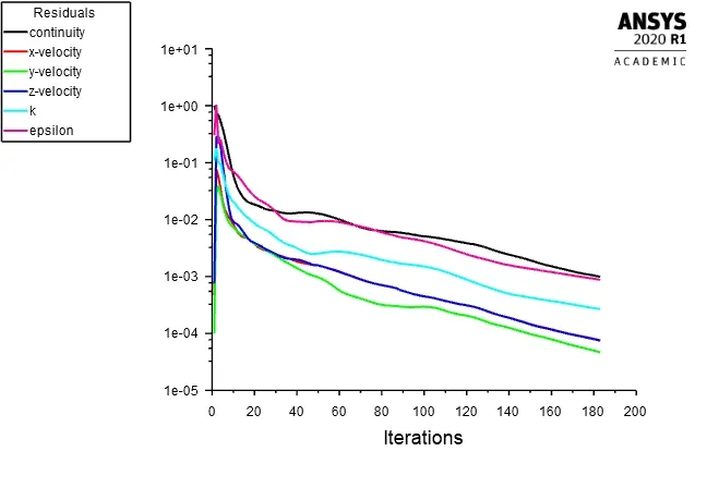
Particle Residence Time:
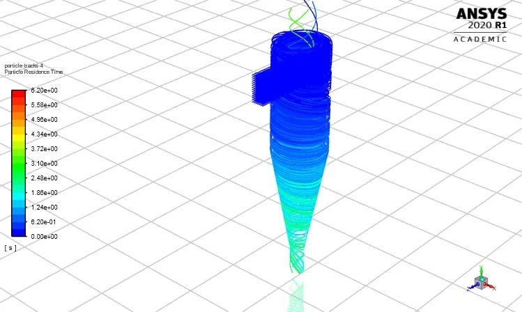
Particle Tracking:

Separation Efficiency in % = (90 / 98) * 100
Separation Efficiency = 91.8 %
(E). Particle Diameter=5 μm
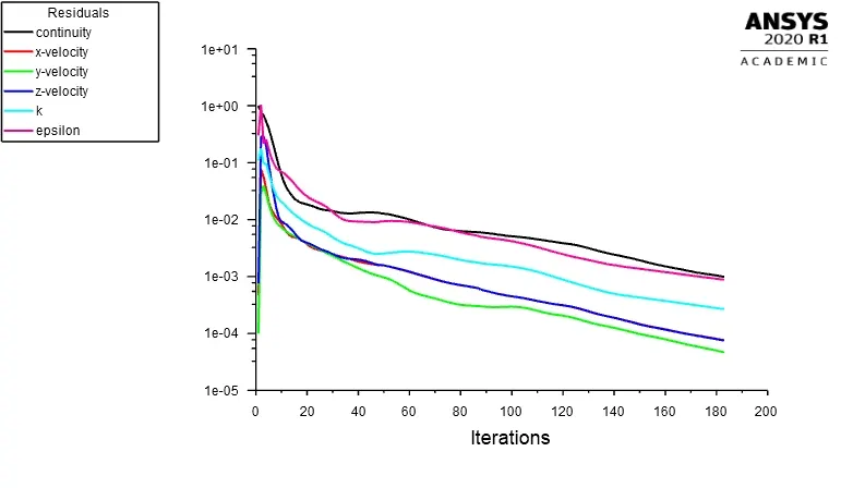
Residual Plots:
Particle Residence Time:
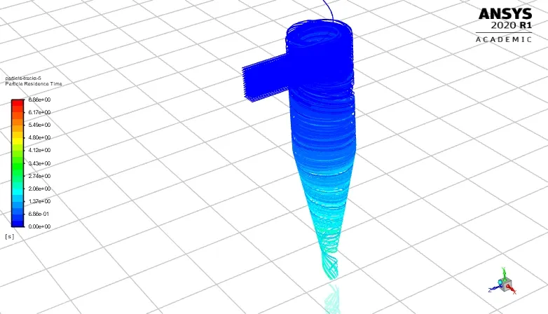
Particle Tracking:

Separation Efficiency in % = (91 / 98) * 100
Separation Efficiency = 92.8 %
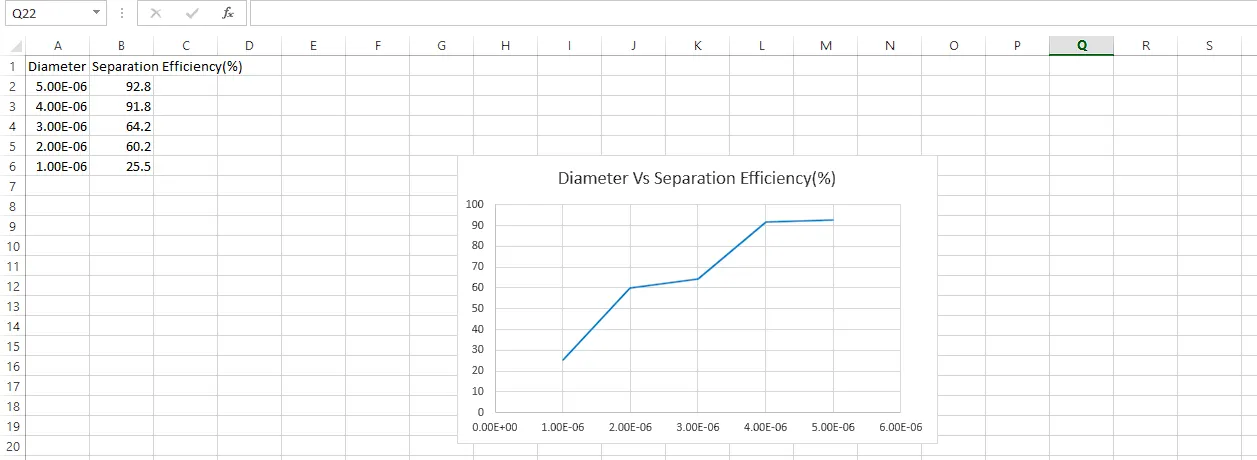
Plot for Diameter vs Separation Efficiency:
Case2:
Particle diameter size=5 μm.
varying the particle velocity from 1 m/sec to 5 m/sec.
(A). Particle velocity=1 m/sec
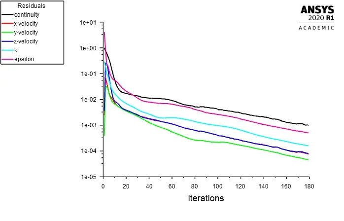
Residual Plots:
Particle Residence Time:
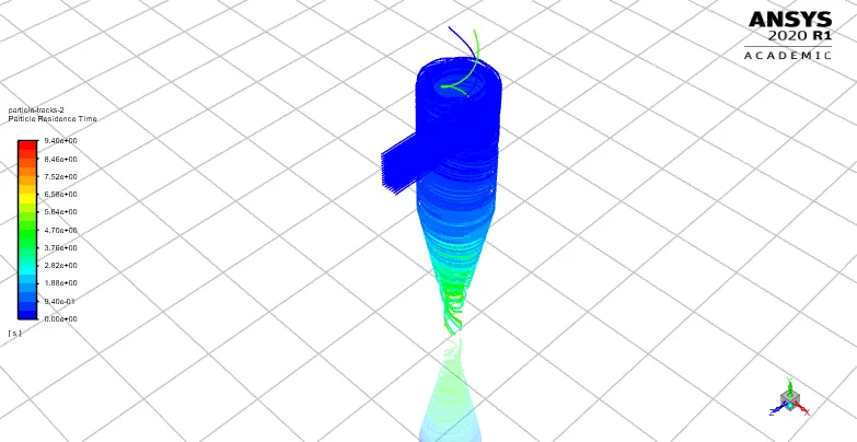
Particle Tracking:

Separation Efficiency in % = (3 / 98) * 100
Separation Efficiency = 3.06 %
Pressure Contour:
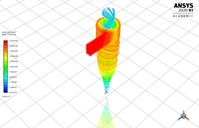
Inlet Pressure=3.05Pa
Outlet Pressure=0.33Pa
Net Pressure=Inlet Pressure-Outlet Pressure=2.72Pa.
(B). Particle velocity=2 m/sec
Residual Plots:
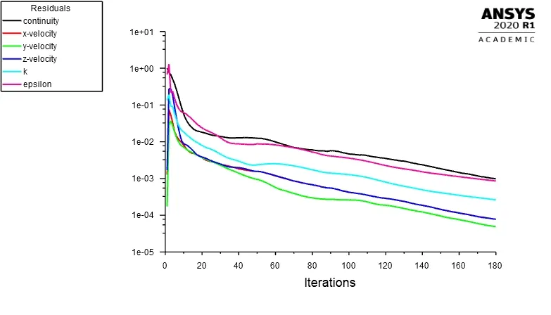
Particle Residence Time:
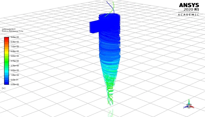
Particle Tracking:

Separation Efficiency in % = (42 / 98) * 100
Separation Efficiency = 42.8 %
Pressure Contour:
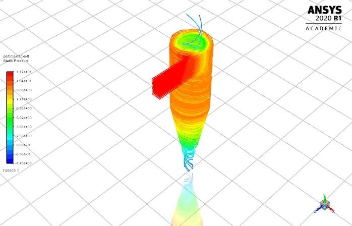
Inlet Pressure=13.70Pa
Outlet Pressure=1.533Pa
Net Pressure=Inlet Pressure-Outlet Pressure=12.17Pa.
(C). Particle velocity=3 m/sec
Residual Plots:
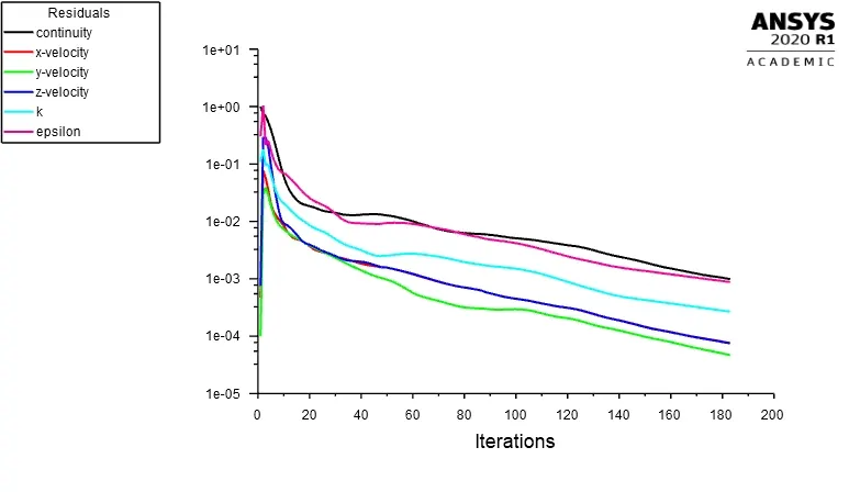
Particle Residence Time:
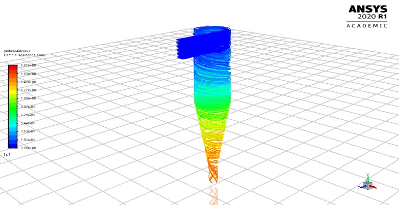
Particle Tracking:

Separation Efficiency in % = (91 / 98) * 100
Separation Efficiency = 92.8%
Pressure Contour:
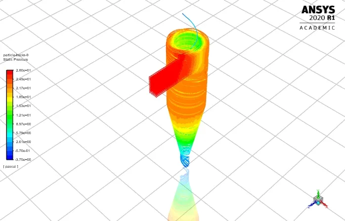
Inlet Pressure=32.33Pa
Outlet Pressure=3.61Pa
Net Pressure=Inlet Pressure-Outlet Pressure=28.72Pa.
(D). Particle velocity=4 m/sec
Residual Plots:
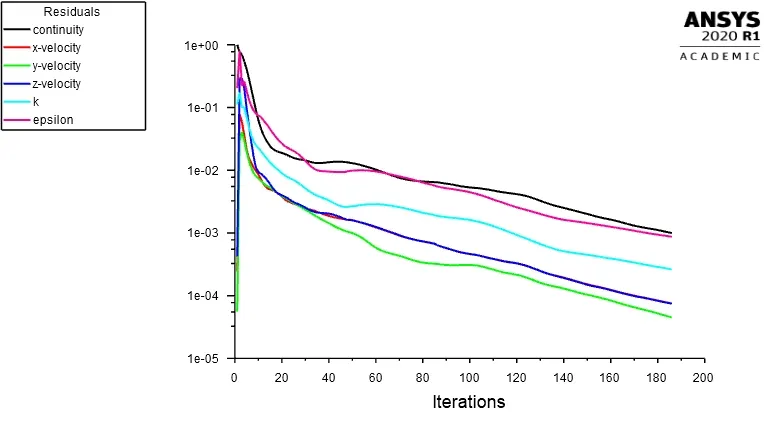
Particle Residence Time:
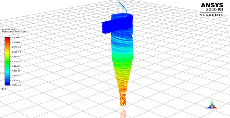
Particle Tracking:

Separation Efficiency in % = (96 / 98) * 100
Separation Efficiency = 97.9%
Pressure Contour:
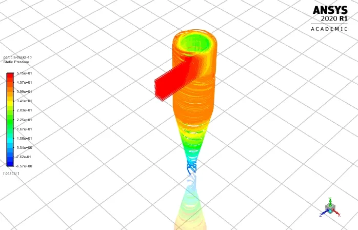
Inlet Pressure=59.00Pa
Outlet Pressure=6.59Pa
Net Pressure=Inlet Pressure-Outlet Pressure=52.41Pa.
(E). Particle velocity=5 m/sec
Residual Plots:
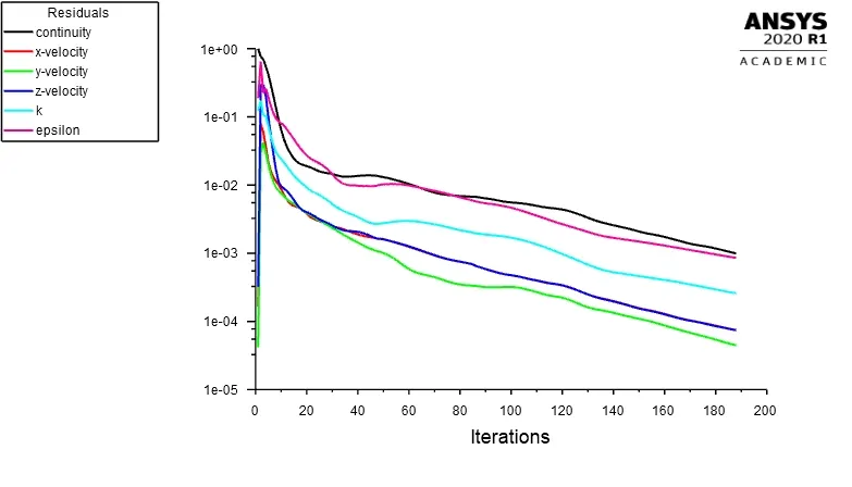
Particle Residence Time:
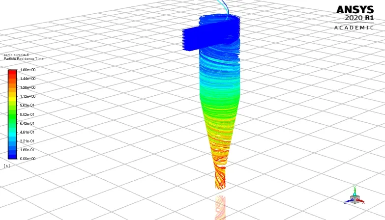
Particle Tracking:

Separation Efficiency in % = (97 / 98) * 100
Separation Efficiency = 98.5%
Pressure Contour:
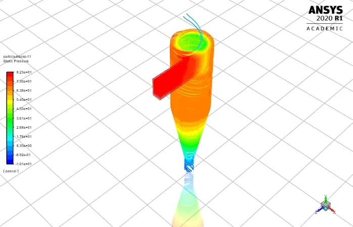
Inlet Pressure=93.8Pa
Outlet Pressure=10.50Pa
Net Pressure=Inlet Pressure-Outlet Pressure=83.3Pa.
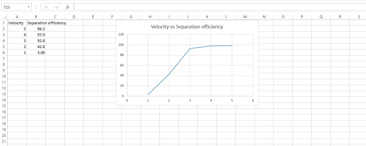
Plot for Velocity vs Separation Efficiency:
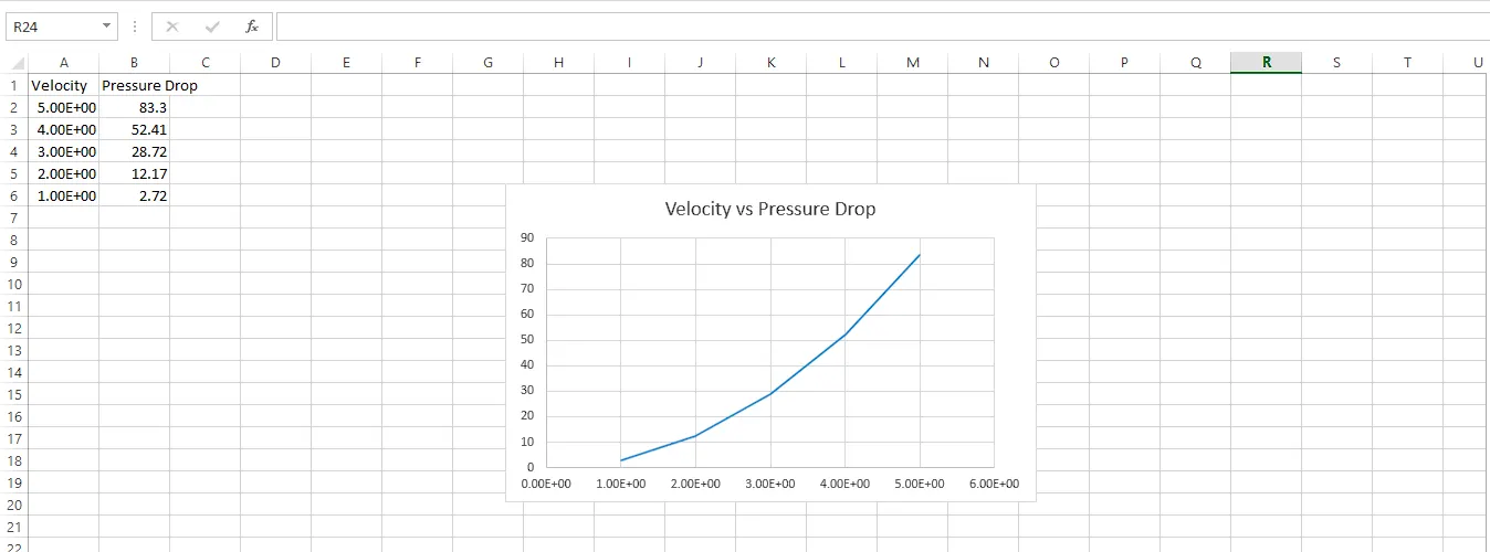
Plot for Velocity vs Pressure Drop:
Conclusions:
1. An increase in diameter and velocity separation efficiency increases.
2. Separation Efficiency depends on both the diameter and velocity of particles.
3. An increase in velocity causes the pressure to drop to rise exponentially.
4. The pressure drop is dependent on the velocity. For constant velocity with varying diameter sizes, the pressure drop remains almost constant.
5. Velocity has a greater impact as compared to the diameter of the particle.
References:
https://skill-lync.com/knowledgebase/theory-guide-for-discrete-phase-modelling
https://www.sciencedirect.com/science/article/pii/S0307904X06000291