Ahmed Body Challenge
Objective: To perform a grid independency test on Ahmed Body.
Expected Results:
1. Velocity and pressure contours.
2. The drag coefficient plot for a refined case. ( For velocity of 25m/sec, the drag coefficient should be around 0.33).
3. The vector plot clearly showing the wake region.
4. Perform the grid independency test and provide the values of drag and lift with each case.
Theory:
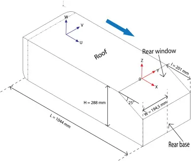
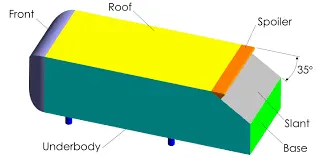
The Ahmed Body is a generic car body or a simplified Automotive vehicle model. The essential flow has been captured by the airflow around the Ahmed body which features around an automobile and was first defined and characterized in the experimental work of S.R. Ahmed. Although it has a very simple shape, the Ahmed body allows us to capture characteristic features that are relevant to bodies in the automobile industry. This model is also used to describe the turbulent flow field around a car-like geometry. Once the numerical model is validated, it is used to design new models of the car.
The main goal of the automotive industry to reduce drag, keeping noise to a minimum, preventing lift (unwanted), and avoiding other unwanted instabilities that can occur at high speeds. Drag is a result of pressure differences between the frontal and the rear end of the vehicle. To reduce drag modifications of the vehicle design or modifications of the airflow around the vehicle. To conduct sufficient aerodynamic analysis in order to observe the behavior of turbulence and pressure, a simplified Ahmed body model will be analyzed. The body is a simplified bluff body that maintains a degree of accuracy when modeling airflow around the vehicle while maintaining great vehicle features.
Two distinct regions created when the air tends to curl downwards at the rear of the vehicle.
(1).High Pressure under the vehicle
(2).Low pressure on the top
While the airflow passed on the rear of the vehicle, there will be collisions or interactions of both pressure results in a wake region. Kinetic energy from these turbulent air interactions tends to act in a direction which is opposite to the direction of the travel. The resultant car engine has to compensate energy losses as a result of Drag. During the flow separation period, vortices are created downstream forming either Structured or UnStructured wake patterns. Region of recirculation flow immediately behind a body that is caused by Viscosity is known as the Wake region. The aerodynamic forces created on a vehicle area as a result of various complex interactions between the flow separations and vortex wake's dynamic behavior.
Importance of Ahmed-Body:
The research of three-dimensional flow around a vehicle has become a subject of significant importance in the Automotive industry. One apparent technique of improving the fuel efficiency of vehicles is to reduce aerodynamic drag force by optimizing the body shape. Execution of fine aerodynamic design under stylistic constraints requires an immense understanding of the flow pattern phenomena and, especially, how the aerodynamics are impacted by changes in body shape.
Ahmed Body was one such generic bluff body proposed to study the external aerodynamics of the vehicles. The flow around the Ahmed body has several flow separations from the front to the rear of the vehicle. The flow recirculation caused by these flow detachment contributes the vehicle’s drag. The location point at which the flow separates determines the size of the separation zone, and accordingly the drag force, thus an exact simulation of the wake flow and of the separation process is essential for the accurate result of drag predictions.
The wake separation flow behind the Ahmed body is the main contributor to the drag force, accurate prediction of the separation process and the wake flow are the key to the successful modeling of this case.
Outcomes for the modeling and Simulation of Ahmed Body:
Consider a fluid particle flows withing the boundary layer around the circular cylinder. From pressure distribution measured, the pressure is a maximum at the stagnation point and gradually decreases along the front half of the cylinder. The flow stays attached in this favorable pressure region as expected. However, the pressure starts to increase in the rear half of the cylinder and the particle now experiences as an adverse pressure gradient. Consequently, the flow separates from the surface and creating a highly turbulent region behind the cylinder called 'WAKE'. The pressure inside the wake region remaining low as the flow separates and a net pressure force (pressure drag) is produced.
Flow Separation:
The presence of the fluid viscosity slows down the fluid particles very close to the solid surface and forms a thin slow-moving fluid layer called a boundary layer. The flow velocity is zero at the surface to satisfy the no-slip boundary condition. Inside the boundary layer, flow momentum is quite low since it experiences a strong viscous flow resistance. Therefore, the boundary layer flow is sensitive to the external pressure gradient (as the form of a pressure force acting upon fluid particles). If the pressure decreases in the direction of the flow, the pressure gradient is said to be favorable. In this case, the pressure force can assist the fluid movement and there is no flow retardation. However, if the pressure is increasing in the direction of the flow, an adverse pressure gradient condition as so it is called exist. In addition to the presence of a strong viscous force, the fluid particles now have to move against the increasing pressure force. Therefore, the fluid particles could be stopped or reversed, causing the neighboring particles to move away from the surface. This phenomenon is called the boundary layer separation.
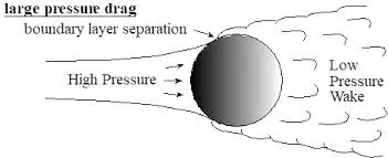
The pressure gradient is an is one of the factors that influence a flow immensely. As discussed above, A negative pressure gradient is termed a Favourable pressure gradient. Such a gradient enables the flow. A positive pressure gradient has the opposite effect and is termed the Adverse Pressure Gradient. Fluid might find it difficult to negotiate an adverse pressure gradient. Sometimes, we say the fluid has to climb the pressure hill. One of the severe effects of an adverse pressure gradient is to separate the flow.
Consider flow past a curved surface as shown in Fig. The geometry of the surface is such that we have a favorable gradient in pressure to start with and up to a point P. The negative pressure gradient will counteract the retarding effect of the shear stress (which is due to viscosity) in the boundary layer. For geometry considered we have an adverse pressure gradient downstream of P.
Now the adverse pressure gradient begins to retard. This effect is felt more strongly in the regions close to the wall where the momentum is lower than in the regions near the free stream. As indicated in the figure, the velocity near the wall reduces and the boundary layer thickens. Continuous retardation of flow brings the wall shear stress at the point S on the wall to zero. From this point onwards the shear stress becomes negative and the flow reverses and a region of recirculating flow develops. We see that the flow no longer follows the contour of the body. We say that the flow has separated. The point S where the shear stress is zero is called the Point of Separation.
Modeling of Ahmed-Body:
While calculating area: (Keep Ahmed Body in front-facing direction)
A=(0.288*0.389)+2*(0.05*0.03).. (2 times because two legs visible at front side)
2.Import the geometry to Ansys SpaceClaim:
3. From a bigger computational domain using the Enclosure option in Spaceclaim as per the below dimension.
The bigger enclosure will be:
4. Our geometry of Ahmed body is perfectly symmetric so using Split Body option in Spaceclaim allows us to reduce nos. of cells and brings out an accurate result using lesser nos. of cells at a lower computational time. Here, we are simulating only half of the complete domain.
Domain after Split Body: After unclicking on Ahmed-Body:
Step2: Mesh
Start with BaseLine Mesh to checkup the setup
(After Section-Plane)
Also, Provide Boundary Names:
Step3: Fluent-Setup
check the mesh first and after that define the solver. Here we used the density-based solver in steady-state simulation because mach is greater than 0.3 and for this condition, density-based solvers give a much accurate result as compared to the pressure-based solvers.
Viscous Model-
We are here working on velocity i.e. 25m/s. Reynold's number also will be higher hence adding the Turbulence model is our necessity.
Checked Energy equation.
Model - K-epsilon (2 equations)
K-epsilon model- Standard
Near-wall Treatment- Standard wall functions
Material- Air with default properties.
Boundary Conditions-
Inlet- Type= Velocity inlet
Velocity Magnitude= 25 m/s
Temperature= 300 K
Outlet- Type= Pressure outlet
Gauge Pressure= 0 Pa
Symmetry- Type= Symmetry
Walls- Type= Wall
Wall Motion= Stationary wall
Shear conditon= No slip
Roughness model= Standard
Results:
Residual plot:
Velocity-contour plot:
Pressure-contour plot:
CoEfficient of Drag: 0.39
CoEfficient of Lift: 0.29
Step-4: Post-Processing
Pressure-contour:
Velocity-contour:
Vector representation of velocity:
Velocity plots for different positions:
Since we run the set-up for a baseline mesh we get the expected results as shown above but as we study on the velocity contour and velocity vector, we get some diffused solution because of the unstructured mesh also get the velocity vectors in some unexpected regions. In computational fluid dynamics, we are very sensitive to selecting the correct meshing which mainly depends on the element size. Normally we did a mesh sensitivity study and after getting the appropriate residual graph for convergence we take it for the problem.Also, there is 62.5% error in the drag coefficient.
(c) Face Meshing:
For Ahmed Body Meshing, Define element size as 15mm
d) Face Meshing:
When we define the element size for enclosure 2 then we get that the shape of the Ahmed body leg turns to pentagon type. So here we defined element size=5 mm to stable in their circular shape.
(e)Inflation:
It is a very important phenomenon for refining a mesh near the wall center of the elements, which does not lie in a single line and we don't get the proper information near the walls. So here we used the boundary layer phenomenon. Using the appropriate boundary layer thickness, we can create the boundary layers.
First, calculate the first layer thickness using the Y+ value for a given velocity, area, density, and viscosity value. We can choose y+ value between 30-300 for k-epsilon with a standard wall function turbulence model. For getting the correct y+ we should run the simulation and compare the coefficient of drag value from the experimental data. If the error is less than 30% in the coefficient of drag so that we can choose the desired y+ for calculation of the first layer thickness. In our case, we choose y+ 100 to start our simulation.
First layer thickness: 1.47mm
No of inflation layers: 5
Total thickness: 3.65 mm.
Step3: Fluent-Setup:
Viscous Model-
We are here working on velocity i.e. 25m/s. Reynold's number also will be higher hence adding the Turbulence model is our necessity.
Checked Energy equation.
Model - K-epsilon (2 equations)
K-epsilon model- Standard
Near-wall Treatment- Standard wall functions
Material- Air with default properties.
Boundary Conditions-
Inlet- Type= Velocity inlet
Velocity Magnitude= 25 m/s
Temperature= 300 K
Outlet- Type= Pressure outlet
Gauge Pressure= 0 Pa
Symmetry- Type= Symmetry
Walls- Type= Wall
Wall Motion= Stationary wall
Shear conditon= No slip
Roughness model= Standard
Results:
Residual plot:
Velocity-contour plot:
Pressure-contour plot:
Coefficient of Drag:0.36
CoEfficient of Lift:0.31
Step-4: Post-Processing
Pressure-contour:
Velocity-contour:
Vector representation of velocity:
Velocity plots for different positions:
Pressure plots for different positions:
Line position for the velocity plots:
c) Face Sizing
When we define the element size for enclosure 2 then we get that the shape of the Ahmed body leg turns to pentagon type. So here we defined element size=4 mm to stable in their circular shape.
d) Inflation
First layer thickness: 1.47mm (Y+ 100)
No of inflation layers: 5
Total thickness: 3.65mm
Fluent-Setup:
Viscous Model-
We are here working on velocity i.e. 25m/s. Reynold's number also will be higher hence adding the Turbulence model is our necessity.
Checked Energy equation.
Model - K-epsilon (2 equations)
K-epsilon model- Standard
Near-wall Treatment- Standard wall functions
Material- Air with default properties.
Boundary Conditions-
Inlet- Type= Velocity inlet
Velocity Magnitude= 25 m/s
Temperature= 300 K
Outlet- Type= Pressure outlet
Gauge Pressure= 0 Pa
Symmetry- Type= Symmetry
Walls- Type= Wall
Wall Motion= Stationary wall
Shear conditon= No slip
Roughness model= Standard
Results:
Residual plot:
Velocity-contour plot:
Pressure-contour plot:
Coefficient of Drag:0.34
CoEfficient of Lift:0.30
Post-Processing:
Pressure-contour:
Velocity-contour:
Vector representation of velocity:
Velocity plots for different positions:
Pressure plots for different positions:
Line position for the velocity plots:
a) Multizone with quad-dominant elements.
Use the element size =70mm
b) Body Sizing
For enclosure 2 use the 38mm element size.
c) Face Sizing
When we define the element size for enclosure 2 then we get that the shape of the ahmed body leg turns to pentagon type. So here we defined element size=5mm to stable in their circular shape.
d) Inflation
First layer thickness: 1.47mm (Y+ 100)
No of inflation layers: 5
Total thickness: 4.38 mm
Fluent-Setup:
Viscous Model-
We are here working on velocity i.e. 25m/s. Reynold's number also will be higher hence adding the Turbulence model is our necessity.
Checked Energy equation.
Model - K-epsilon (2 equations)
K-epsilon model- Standard
Near-wall Treatment- Standard wall functions
Material- Air with default properties.
Boundary Conditions-
Inlet- Type= Velocity inlet
Velocity Magnitude= 25 m/s
Temperature= 300 K
Outlet- Type= Pressure outlet
Gauge Pressure= 0 Pa
Symmetry- Type= Symmetry
Walls- Type= Wall
Wall Motion= Stationary wall
Shear conditon= No slip
Roughness model= Standard
Results:
Residual plot:
Velocity-contour plot:
Pressure-contour plot:
Coefficient of Drag:0.332
CoEfficient of Lift:0.29
Post-Processing:
Pressure-contour:
Velocity-contour:
Vector representation of velocity:
Velocity plots for different positions:
Pressure plots for different positions:
Line position for the velocity plots: