Steady Vs Unsteady flow over a cylinder

Objective: Simulate the flow over a cylinder and explain the phenomenon of Karman vortex street.

PART-I: Simulate the flow with the steady and unsteady case and calculate the Strouhal Number for Re= 100.

PART-II: Calculate the coefficient of drag and lift over a cylinder by setting the Reynolds number to 10,100,1000,10000 & 100000. (Run with steady solver).

Discuss the effect of Reynolds number on the coefficient of drag. [ Results should be validated with any standard literature and error should be within 5 %]

Expected results:

1. In both approaches, show that the flow has converged. That is, what quantities or plots need to be looked at to determine that the flow has converged?
2. Plots of the coefficient of drag and lift.
3. Plots to show vortex shedding behind the cylinder.

Given:

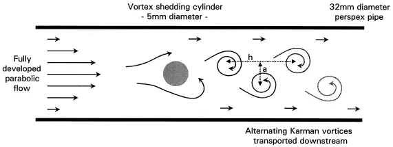
The Computational domain which we are going to create as shown below:

Cylinder diameter(D):2m.

Total length=30D.

Height=10D.

Viscosity=0.05 Kg/ms

Theory:

The phenomenon of Karman vortex

In Fluid Dynamics, a Karman vortex street is a repeating pattern of swirling vortices, caused by a process known as Vortex Shedding, which is responsible for the unsteady separation of Fluid around blunt bodies. It is named after the engineer and fluid dynamicist Theodore Von Karman.

Vortex shedding is a phenomenon when the wind blows across a structural member, vortices are shed alternately from one side to the other, and where alternating low-pressure zones are generated on the downwind side of the structure giving rise to a fluctuating force acting at right angles to the wind direction.

Vortices are a major component of turbulent flow. The distribution of velocity, vorticity (the curl of the flow velocity), as well as the concept of circulation is used to characterize vortices. In most vortices, the fluid flow velocity is greatest next to its axis and decreases in inverse proportion to the distance from the axis.

For common flows (the ones which can usually be considered as incompressible or isothermal), the kinematic viscosity is everywhere uniform over all the flow field and constant in time, so there is no choice on the viscosity parameter, which becomes naturally the kinematic viscosity of the fluid being considered. On the other hand, the reference length is always an arbitrary parameter, so particular attention should be put when comparing flows around different obstacles or in channels of different shapes: the global Reynolds numbers should be referred to the same reference length. This is actually the reason for which most precise sources for airfoil and channel flow data specify the reference length at a prefix to the Reynolds number. The reference length can vary depending on the analysis to be performed: for a body with circle sections such as circular cylinders or spheres, one usually chooses the diameter; for an airfoil, a generic non-circular cylinder or a bluff body or a revolution body like a fuselage or a submarine, it is usually the profile chord or the profile thickness, or some other given widths that are in fact stable design inputs; for flow channels usually, the hydraulic diameter about which the fluid is flowing.

For an aerodynamic profile, the reference length depends on the analysis. In fact, the profile chord is usually chosen as the reference length also for the aerodynamic coefficient for wing sections and thin profiles in which the primary target is to maximize the lift coefficient or the lift/drag ratio (i.e. as usual in thin airfoil theory, one would employ the chord, Reynolds, as the flow speed parameter for comparing different profiles). On the other hand, for fairings and struts the given parameter is usually the dimension of internal structure to be streamlined (let us think for simplicity it is a beam with circular section), and the main target is to minimize the drag coefficient or the drag/lift ratio. The main design parameter which becomes naturally also a reference length is therefore the profile thickness (the profile dimension or area perpendicular to the flow direction), rather than the profile chord.

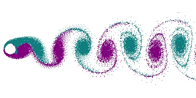
The range of Re values will vary with the size and shape of the body from which the eddies are being shed, as well as with the kinematic viscosity of the fluid. Over a large Re range (47<Re<10⁵ for circular cylinders; reference length is d: diameter of the circular cylinder) eddies are shed continuously from each side of the circle boundary, forming rows of vortices in its wake. The alternation leads to the core of a vortex in one row being opposite the point midway between two vortex cores in the other row, giving rise to the distinctive pattern shown in the picture. Ultimately, the energy of the vortices is consumed by viscosity as they move further downstream, and the regular pattern disappears.

When a single vortex is shed, an asymmetrical flow pattern forms around the body and changes the pressure distribution. This means that the alternate shedding of vortices can create periodical lateral (sideways) forces on the body in question, causing it to vibrate. If the vortex shedding frequency is similar to the natural frequency of a body or structure, it causes resonance.

Some of the real-life examples of Vortex shedding are:

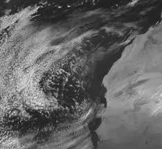
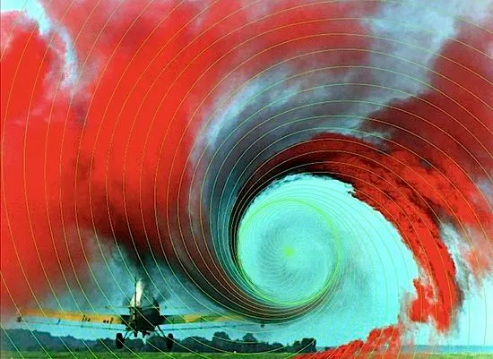
Physics behind Vortex formation:

As a Fluid particle flows towards the leading edge of a cylinder, the pressure on the particle rises from the free stream pressure to stagnation pressure. The high fluid pressure near the leading edge impels flow about the cylinder as a boundary layer develops about both sides. The high pressure is not sufficient to force the flow about the back of the cylinder at high Reynolds number. Near the widest section of the cylinder, the boundary layer separates from each side of the cylinder surface and form 2 shear layers. Since the innermost portion of the shear layers, which is in contact with the cylinder, moves much more slowly than the outermost portions of the shear layers which is in contact with the free flow, the shear layers roll near the wake.

Understanding the physics behind vortex shedding is quite important from an engineering point of view. For example, if the bluff structure is not mounted rigidly and the frequency of vortex shedding matches the resonance frequency of the structure, then the structure can begin to resonate and starts vibrating. These vibrations can cause severe damage to the structure.

Case Setup:

In order to simulate flow over a cylinder, Following steps need to be followed:

1. Geometry Formation.
2. Mesh Generation.
3. SetUp Fluent case.
4. Post-Processing.

1. Geometry Formation/Create a Computational Domain:

As a 2D Computational domain shown above, we have to create a 2D designing inside a Spaceclaim using tools like Construction lines, circles, rectangles.

2. Mesh Generation:

Method: Initially, Ansys Meshing creates a quadrilateral dominant mesh, we need to convert it into a triangle dominant mesh.

Go to Mesh > Insert > Method > Select Face > Method(Triangles) > Generate Mesh

Here for all case studies, we will be using Mesh Size of 0.2m.

Sizing: The cylinder we have is not perfectly circular, so if we proceed like that geometry might be inaccuracy in results. This option will help us to create smooth curves by dividing the circle into a large number of edges.

Go to sizing > Select edge > Type(Number of divisions) > Enter number and generate mesh.

Geometry: Select the circle by selecting the edge.

Type: Number of Divisions.

A number of Divisions:36 numbers(360/10).

Growth rate:1.2

Inflation: In order to resolve the boundary over the cylinder We require finner mesh around the cylinder. This option will let us create a finner "body-fitted mesh" as the flow around the cylinder is quite important. Select Geometry: Select Face

*Boundary scooping method: Select circle

*Inflation option: First layer thickness of the 5e-3m thickness

*Maximum layers: 6

*Growth rate:1.2

Boundary Naming: Naming will be done as below.

3. Fluent SetUp:

>First run and perform check mesh in order to find any errors in the geometry.

*Physics:

General:

• Solver: Pressure based
• Velocity formulation: Absolute
• Time: Based on the case study we are going to do(Steady/UnSteady)
• 2D Space: Planar

Model:

Viscous model- Laminar

Materials:

• Create: User_defined_fluid(The fluid is created such that only velocity will be responsible for varying Reynold's number)
• Name:User_defined_fluid

Properties:Density(Kg/m3)=1(constant) Viscosity(Kg/m-s)=0.05(constant) Velocity(m/s)=n(constant)

Where 'n' depends on the Reynolds Number.

Reynolds no, Re = ( [ ρ*u*D ] / μ )

Table:

Boundaries:

Inlet-Velocity inlet(Velocity magnitude):n(m/s).

Outlet-pressure outlet(Gauge pressure):0Pa.

Symmetry-Symmetry(Zone name):Symmetry.

Walls wall >Wall motion: Stationary wall.

Shear condition: No slip.

Solutions:

Create a vertex average of velocity magnitude using surface report at a monitor point 8D from the center of the cylinder to the right of the cylinder along the X-direction.

Coefficient of drag and Coefficient of lift using force report.

Initialization method: Hybrid for Steady-State simulations.

The standard for UnSteady-State simulations.

Activities: Contour plots of pressure and velocity, and solution animation needs to create after initializing the solution.

Run Calculation:

For Steady-State:No. of iterations=350

For Transient-state: Timestep size of 0.1 sec for No of time steps of 500.

Part-1:

In this case study flow over cylinder has been presented where Re No taken as 100 for both Steady and UnSteady state simulations.

Results: For Steady State

In Steady State, Consider No of iterations as 350 and velocity=2.5m/s for Re=100.

Residual plots:

From the above graph, We can see, the solution has reached a steady-state even much before 350 iterations.

Coefficient of Drag and Coefficient of Lift plot:

Coefficient of Drag:
The aerodynamic drag coefficient is a measure of the effectiveness of a streamline aerodynamic body shape in reducing the air resistance to the forward motion of a vehicle. A low drag coefficient implies that the streamline shape of the vehicle's body is such as to enable it to move easily through the surrounding viscous air with the minimum of resistance; conversely, a high drag coefficient is caused by poor streamlining of the body profile so that there is a high air resistance when the vehicle is in motion.

Cd is given by, Cd=2Fd/ρ⋅u^2⋅A

where, Fd- implies to the Net backward force

Coefficient of Lift:
The lift coefficient (C_L) is a dimensionless coefficient that relates the lift generated by a lifting body to the fluid density around the body, the fluid velocity, and an associated reference area.

Cl is given by, Cl=2Fl/ρ⋅u^2⋅A

where, Fl- implies to the Net Upward force

Contour Plot:

Pressure contour plot:

Velocity contour plot:

Vertex average of velocity magnitude:

Results: For Transient State

In the Transient case, we will be stimulating with a Timestep size of 0.1 sec for No of time steps of 500.
Velocity 2.5 m/s for Re. no.100.

Residual plots:

Coefficient of Drag and Coefficient of Lift plot:

Velocity contour plot:

Pressure contour plot:

Vertex average of velocity magnitude:

Strouhal Number:

In dimensional analysis, the Strouhal number (Sr) is a dimensionless number describing oscillating flow mechanisms.
The Strouhal number represents the ratio of inertial forces due to the local acceleration of the flow to the inertial forces due to the convective acceleration. Depending on the time scale of the problem, this ratio may be of order unity, and therefore its importance is not obvious.

Thus, an alternative definition of the Strouhal number better suited to periodic flows is given by the following expression:

St=f⋅L/U

Where, f - Frequency of vortex shedding/oscillations
L- Characteristics length
U- Flow velocity

For Steady-state,

We cannot calculate the frequency parameter in Steady-state simulations as there is no time parameter involved.

For Transient State,

Flowtime- 20
Nos. of peaks or falls= 3

f=3/20

f=0.15 Hz

Therefore, Strouhal no. is

St=0.15*2/1

St=0.3.

Part-2: STEADY FLOW WITH Re - 10,100,1000,10000,100000.

CASE 1:-Steady flow Re 10.

(Tried 700 iterations too, So as to check whether it remains same or not)

CASE 2:-Steady flow Re 100.

CASE 3:-Steady flow Re 1000.

CASE 4:-Steady flow Re 10000. (400 Iterations)

CASE 5:-Steady flow Re 100000. (400 Iterations)

Conclusions:

In the above results, We can predict that as Reynolds number increases Drag coefficient decreases

(1).Flow is converging in both the steady and unsteady state simulations for Reynolds number=100. But, to effectively calculate the Straouhal Number Transient simulation is better as compared to steady-state as it gives a solution at every time step.
(2).For very low Reynolds numbers such as 10 in this case, Vortex does not get generated as Pressure is too high(low velocity too) in that case.
(3).As the cylinder is a bluff body, from the contour of velocity we can conclude that flow remains separated after the cylinder.
(4).From the Reynolds number vs Coefficient of Drag plot, we can conclude that drag is reducing as the Reynolds number is increasing. As the Reynolds number increases, the pressure decreases, and for both a laminar and a turbulent boundary layer increasing Reynolds Number gives lower skin friction drag. Hence, the drag coefficient decreases with an increase in the Reynolds number.