Exhaust Port Challenge
Aim: Observing the thermal behaviour of a hot fluid flowing through the exhaust pipe, and obtaining an accurate value of the Heat Transfer Coefficient on the internal solid surface of the exhaust manifold.
Introduction: Why and Where CHT is used??
The term CHT is used to describe processes which involve variations of temperature within solids and fluids, due to thermal interaction between the solids and fluids. The exchange of thermal energy between the two physical bodies is called the study of heat transfer, the rate of transferred heat is directly proportional to the temperature difference between the bodies. A typical example is the heating or cooling of a solid object by the flow of air in which it is immersed and some other example includes conduction through solids, free and forced convection in the gasses/fluids and thermal radiations.
In natural convection, Any fluid motion is caused by natural means such as the buoyancy effect, i.e. the rise of warmer fluid and fall the cooler fluid. Whereas in forced convection, the fluid is forced to flow over a surface or in a tube by external means such as a pump or fan
Conjugate heat transfer corresponds with the combination of heat transfer in solids and heat transfer in fluids. In solids conduction often dominates, whereas in fluids convection usually dominates. Efficiently combining heat transfer in fluids and solids is the key to designing effective coolers, heaters or heat exchangers. Forced convection is the most common way to achieve a high heat transfer rate. In some applications, the performances are further improved by combining convection with phase change ( for example liquid water to vapour phase change ).
Heat transfer in solids and heat transfer in fluids are combined in the majority of applications. This is because fluid flows around solids or between solids wall and because solids are usually immersed in a fluid.
Conjugate Heat Transfer analysis is used to capture accurate heat transfer behaviour due to both convection and conduction, for cases in which a solid and fluid at different temperatures or subjected to different thermal conditions interact with each other. This is especially useful at the fluid-solid interface, where the fluid interacts thermally with solid. The result obtained is a coupled solution, taking into account the thermal effects due to both, conduction and convection. It is also known for its flexibility, and its ability to handle complex simulations. Conjugate Heat Transfer can be used in a wide range of cases that involve mass-flow of fluid over or inside a solid, subjected to different thermal conditions. Examples of the usage of CHT is seen in the determination of the effectiveness of heat transfer of a solid fin with a fluid flowing around it, fluid flowing through a tube at different temperatures, such as a heat exchanger, and many more applications. A point to note is that CHT is not limited to just conduction and convection, but can take into consideration radiation heat transfer as well.
Forced Convection CHT in Microprocessor CHT in Boiler CHT inside an Inverter
In this particular case, the hot fluid flowing through the exhaust pipe is air, at 700 kelvin. The hot fluid interacts with the solid surface of the pipe, which is at a lower temperature, and the heat transfer at this point is due to convection. The inner wall in contact with the fluid increases in temperature and the heat then flows from the inner wall to the outer wall. The pipe thickness is heated, caused by heat transfer due to conduction. The outer wall of the exhaust pipe is subjected to convection at 20 w/m^2, at 25 degrees Celsius.
Theory:
The exhaust manifold is a vital component in the automotive design of a vehicle, as it is used to collect the exhaust gases formed due to combustion of the fuel and air within the cylinders and provide a path for the gases to escape it to the atmosphere. The exhaust manifold has multiple inlets connected to the exhaust ports on the cylinders in the engine. The high-pressure exhaust gases flow through the pipe with relative ease, as the pressure difference between the exhaust pipe outlet at atmospheric pressure and the high-pressure exhaust gases in the cylinder, is enough for the gases to get sucked out of the combustion chamber.
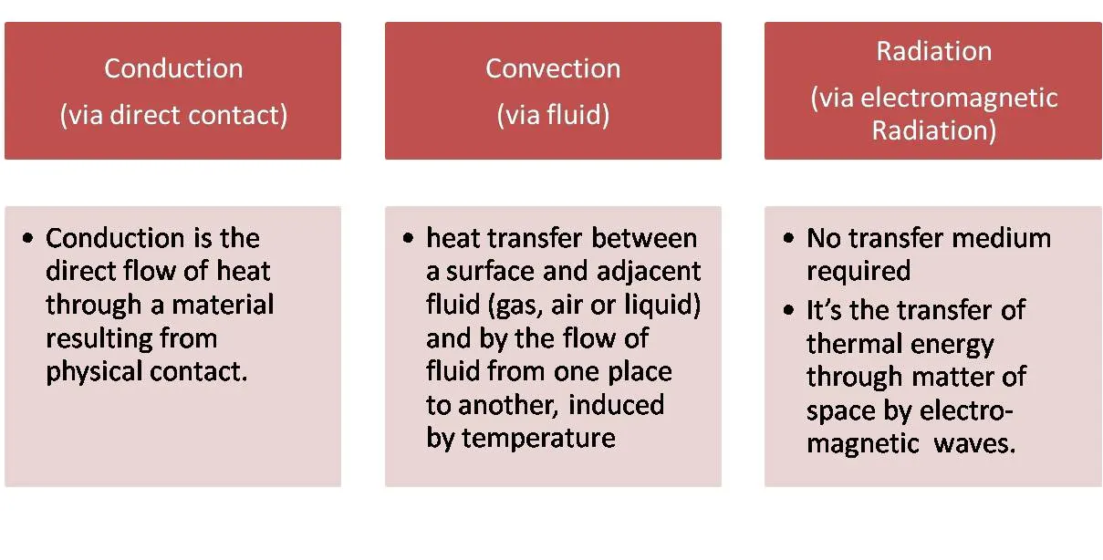
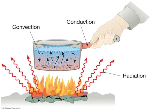
Modes of heat transfer:-
- Conduction:-Diffusion of heat due to temperature gradients. A measure of the amount of conduction for a given gradient is heat conductivity.
- Convection:-When heat is carried away by moving fluids. The flow can either be caused by external influences, forced convection or buoyancy forces, natural convection. Convective heat transfer is tightly coupled to the fluid flow solution.
- Radiation:-Transfer of energy by electromagnetic waves between surfaces with different temperatures, separated by a medium that is at least partially transparent to the (infrared) radiations. Radiation is especially important at high temperatures, for example during combustion processes, but can also have a measurable effect at room temperatures.
CHT in an IC Engine
Conjugate heat transfer:-The term conjugate heat transfer (CHT) is used to describe the processes which involve variations of temperature within solids and fluids due to thermal interaction between the solid and fluids. The exchange of thermal energy between the two physical bodies is called the study of heat transfer, the rate of transferred heat is directly proportional to the temperature difference between the bodies. Conjugate heat transfer corresponds with the combination of heat transfer in solids and heat transfer in fluids. In solids, conduction often dominates. Efficiently combining heat transfer in fluid and solids is the key to designing effective coolers, heaters, or heat exchangers. Forced convection is the most common way to achieve a high heat transfer rate. In some application, the performance is further improved by combining convection with phase change.
We need it because An accurate description of heat transfer modes, material properties, flow regimes, and geometrical configurations enables the analysis of temperature fields and heat transfer.
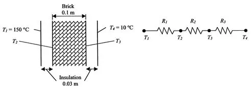
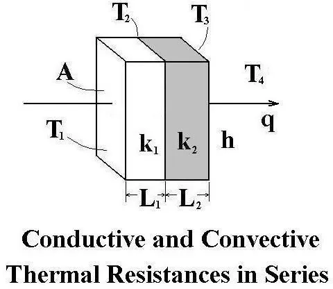
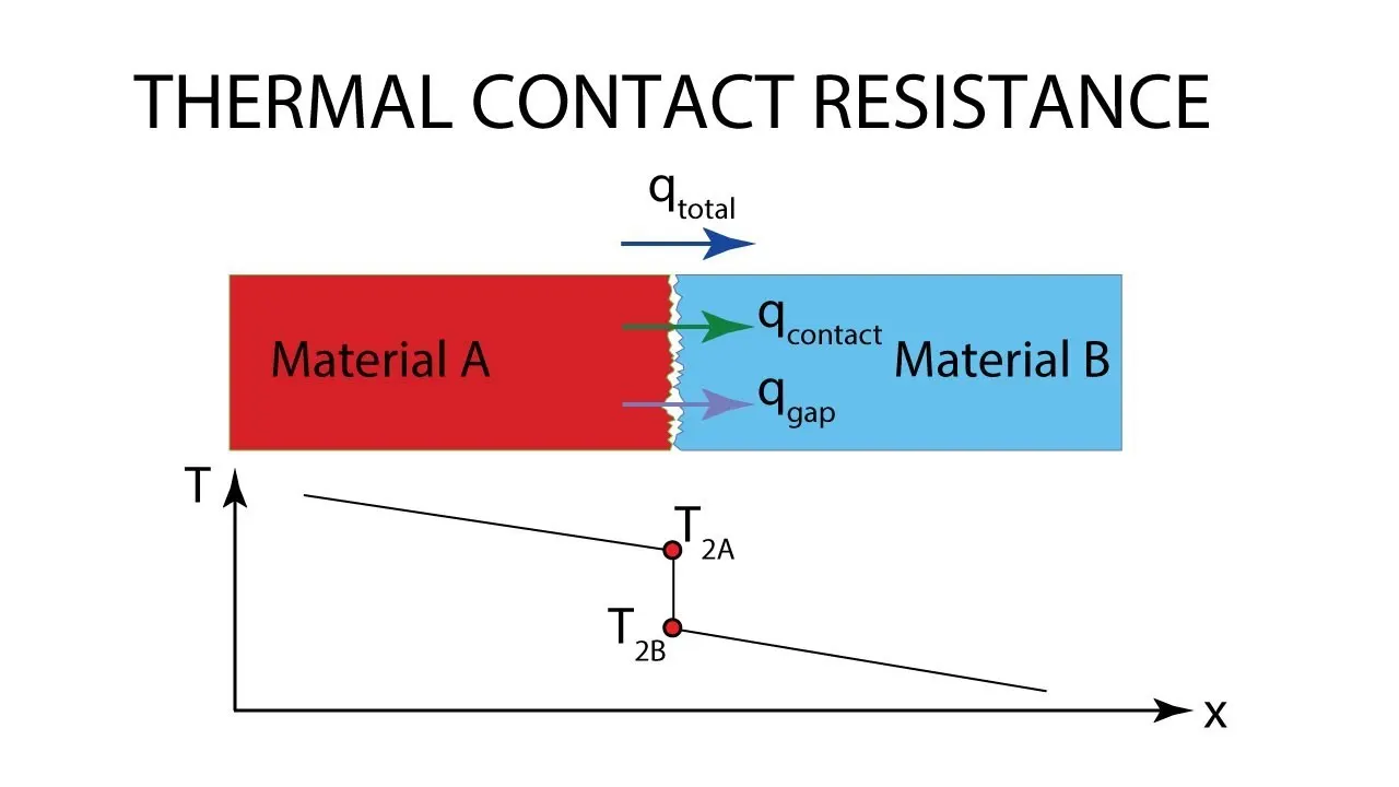
Thermal resistance is defined as the ratio of the temperature difference between the two faces of a material to the rate of heat flow per unit area. Thermal resistance determines the heat insulation property of a textile material. The higher the thermal resistance, the lower is the heat loss or in some case like in radiation resistance heat gain too.
|
Length X |
0.57492 m |
|
Length Y |
1.0619 m |
|
Length Z |
2.7462 m |
|
Properties |
|
|
Volume |
0.13719 m³ |
The above geometry describes the solid part of the component. The fluid domain is extracted from this component:
Exhaust Manifold Geometry with Fluid Domain:
The Exhaust port of in-line four-cylinder engine is created and modified in ANSYS SpaceClaim. In a geometrical model of the exhaust port, a Volume Extract method is used to separate inner fluid volume from the outer solid volume, so that the inner volume can be defined as fluid flowing through the outer solid volume of exhaust port during the time of the simulation.
The solid and fluid volumes are separated in the above geometrical model. When we try to create a base-line mesh, we will find that the common boundary or face between the solid and liquid volume is not properly connected, which can cause an inaccurate result. This type of mesh is known as Non-Conformal Mesh in which nodes of the elements between solid and liquid volume are not connected properly due to which accurate heat transfer will not take place from fluid to solid volume walls and thus, it will give an inaccurate temperature result at solid boundaries.
In order to avoid the above problem and to get Conformal Mesh, we can use Share Topology and Share Prep method from ANSYS SpaceClaim. This method is used to create a smooth interface path between solid and liquid volumes from inlet to outlet and thus, results in a smooth heat transfer and sharing of data between them, which will give an accurate simulation result at solid-fluid volume interface.
Mesh-Details:
Boundary condition definition:
And outer body as"Outer-wall-convection"
Case-1 > Baseline Mesh:
Statistics:
Element type:Tetragonal Mesh
Nodes:27429
Elements:137545
Mesh Quality:
1.Element quality:
- Min:0.14098
- Max:0.99989
- Average:0.81983
- Standard Deviation:0.10038
2.Aspect Ratio:
- Min:1.1676
- Max:14.639
- Average:1.8985
- Standard Deviation:0.49583
3.Skewness:
- Min:2.0426e-004
- Max:0.87347
- Average:0.25068
- Standard Deviation:0.12764
Fluent:
- The k-omega SST model has been designed to combine the advantages of the k-epsilon and k-omega turbulence models. The k-omega model solves the near-wall functions accurately, but is inaccurate in the freestream velocity sections of the fluid flow, whereas the k-epsilon model accurately solves the freestream section of the fluid flow, but provides inaccurate values at the near wall or viscous sub-layer section.
- The k-omega SST model uses a k-epsilon model in the freestream sections of the fluid flow, and a k-omega model for near-wall computations. The ability of the k-omega SST model to resolve near-wall behaviour is imperative to attaining precise thermal behaviour near the inner wall.
- This seamless switching between models is done by the integration of two blending functions 'F1' and 'F2' in the equations of specific dissipation rate and kinematic eddy viscosity respectively.
- If the value of F1 is zero, the model switches to the k-epsilon model. Similarly, if the value of F1 is one, the k-omega model is used.
- F2 involves the use of a viscosity limiter, which prevents the model from over-predicting the wall shear stress, and functions similar to F1.
Pre-processing in Fluent:
- The solver type and the steady-state simulation options are set by going to Setup>General.
- The energy equation is turned on, as it is required in order to simulate heat transfer. This is done by going to Setup> Models > Energy Equation.
- The turbulence model is switched to k-omega SST by going to Setup> Models > Viscous, for the reasons stated above.
- The default fluid in fluent for the fluid is air, so no changes will be made to the material. However, this can be changed by selecting the fluid in Setup>Materials>Fluid, and then changing it in Setup>Cell Zone conditions>Fluid.
Boundary conditions:
- The freestream velocity is set to 5 m/s at the inlet by going into Setup > Boundary Conditions > Inlet. The temperature of the fluid is changed in the same window by going to the Thermal settings in the same window and is set to 700K.
- The thermal boundary conditions of the inner wall are set to the couple.
- The thermal boundary conditions of the outer wall are changed to convection, with the heat transfer coefficient of air set to 20 W/m^2-K.
- The boundary conditions of the simulation are under the same section under 'Type', and can be changed by using the dropdown provided below in the section.
- The boundary conditions are set in Fluent, as shown in the table below.
-
Inlet Velocity-inlet Outlet Pressure-inlet Inner wall wall Outer wall wall Solid interior Fluid interior
Residuals:
Temperature Contour:
Post-Processing:
Temperature at outer wall convection:
Velocity Stream-line:
Heat transfer coefficient at outer-wall-convection:
The temperature at Outer wall-convection:
Velocity Plane:
Pressure Plane:
Temperature Plane:
Case-2 (Refined Mesh)
- For refinement of mesh, we add inflation layers so as to find the accurate near the walls. The thickness of the inflation layer depends on the turbulence model. When we see the Reynolds number, if we take k-epsilon turbulence model the standard wall function y+ range is 30-300 whereas for the k-omega SST model y+ range is 1-5. In a few cases, it may go down below 1.
- As we add inflation layers for refinement, in this case, we take total thickness as 5mm. Further by validating we can either increase or decrease the total thickness as this completely depends on the value of y+.
- Also, we add body sizing for refinement. On adjusting the value here we should maintain the maximum number of elements that we are getting. This is because we have restrictions to the academic version of the software.
- To check the Element Quality go to Details of Mesh > select Quality > click on Mesh Metric. The plot is created to check the quality. In this case, we consider a minimum of 10%. Check for the quality.
Inputs :
Element Size- 150mm(Fluid domain)
Body Sizing- 10mm(Outer Body)
Inflation layers- 5
Total thickness- 5mm(Inflation layer b/w Fluid body to Outer body for CHT)
Velocity Magnitude- 5m/s
Inlet Temperature- 700k
Heat Transfer Coefficient- 20 W/m^2-k.
Fluid domain(Name it as Inflation):(By hiding outer body)
Statistics:
Element type:Tetragonal Mesh
Nodes:120101
Elements:410056
Mesh Quality:
1.Element quality:
- Min:8.4152e-004
- Max:0.99963
- Average:0.53126
- Standard Deviation:0.3206
2.Aspect Ratio:
- Min:1.1737
- Max:1762.1
- Average:59.565
- Standard Deviation:226.82
3.Skewness:
- Min:6.4204e-004
- Max:0.89779
- Average:0.34583
- Standard Deviation:0.2373
Fluent:
Pre-processing in Fluent:
- The solver type and the steady-state simulation options are set by going to Setup>General.
- The energy equation is turned on, as it is required in order to simulate heat transfer. This is done by going to Setup> Models > Energy Equation.
- The turbulence model is switched to k-omega SST by going to Setup> Models > Viscous, for the reasons stated as in Case1.
- The default fluid in fluent for the fluid is air, so no changes will be made to the material. However, this can be changed by selecting the fluid in Setup>Materials>Fluid, and then changing it in Setup>Cell Zone conditions>Fluid.
Boundary conditions:
- The freestream velocity is set to 5 m/s at the inlet by going into Setup > Boundary Conditions > Inlet. The temperature of the fluid is changed in the same window by going to the Thermal settings in the same window and is set to 700K.
- The thermal boundary conditions of the inner wall are set to coupled.
- The thermal boundary conditions of the outer wall are changed to convection, with the heat transfer coefficient of air set to 20 W/m^2-K.
- The boundary conditions of the simulation are under the same section under 'Type' and can be changed by using the dropdown provided below in the section.
- The boundary conditions are set in Fluent, as shown in the table below.
-
Inlet Velocity-inlet Outlet Pressure-inlet Inner wall wall Outer wall wall Solid interior Fluid interior
Residuals:
Temperature Contour:
Y-Plus Plot:
Post-Processing:
The temperature at outer wall convection:
Velocity Stream-line:
Heat transfer coefficient at outer-wall-convection:
The temperature at Outer wall-convection:
Velocity Plane:
Pressure Plane:
Case3>Refined Mesh Inflation:
Use Y+ as 2.5
While calculating length, Calculate from Starting point of the first inlet to the end of the outlet of the Exhaust port(In a Pipe where exhaust gas travels)
-
Inputs :
Element Size- 150mm(Fluid domain)
Body Sizing- 17mm(Outer Body)
Inflation layers- 5
Total thickness- 0.43456mm(Inflation layer bw Fluid body to Outer body for CHT)
Velocity Magnitude- 5m/s
Inlet Temperature- 700k
Heat Transfer Coefficient- 20 W/m^2-k.
Fluid domain(Name it as Inflation):(By hiding outer body)
Statistics:
Element type: Tetragonal Mesh
Nodes:152611
Elements:447228
Mesh Quality:
1.Element quality:
- Min:3.6791e-003
- Max:0.99999
- Average:0.44817
- Standard Deviation:0.41611
2.Aspect Ratio:
- Min:1.1588
- Max:515.05
- Average:101.32
- Standard Deviation:117.18
3.Skewness:
- Min:1.1061e-005
- Max:0.86604
- Average:0.18814
- Standard Deviation:0.11766
Fluent:
Pre-processing in Fluent:
- The solver type and the steady-state simulation options are set by going to Setup>General.
- The energy equation is turned on, as it is required in order to simulate heat transfer. This is done by going to Setup> Models > Energy Equation.
- The turbulence model is switched to k-omega SST by going to Setup> Models > Viscous, for the reasons stated as in Case1.
- The default fluid in fluent for the fluid is air, so no changes will be made to the material. However, this can be changed by selecting the fluid in Setup>Materials>Fluid, and then changing it in Setup>Cell Zone conditions>Fluid.
Boundary conditions:
- The freestream velocity is set to 5 m/s at the inlet by going into Setup > Boundary Conditions > Inlet. The temperature of the fluid is changed in the same window by going to the Thermal settings in the same window and is set to 700K.
- The thermal boundary conditions of the inner wall are set to coupled.
- The thermal boundary conditions of the outer wall are changed to convection, with the heat transfer coefficient of air set to 20 W/m^2-K.
- The boundary conditions of the simulation are under the same section under 'Type', and can be changed by using the dropdown provided below in the section.
- The boundary conditions are set in Fluent, as shown in the table below.
-
Inlet Velocity-inlet Outlet Pressure-inlet Inner wall wall Outer wall wall Solid interior Fluid interior
Residuals:
Temperature Contour:
Y-Plus Plot:
Post-Processing:
The temperature at the outer wall convection:
Velocity Stream-line:
Heat transfer coefficient at outer-wall-convection:
Heat transfer coefficient is 957.7w/(m^2.k)
Velocity Plane:
Pressure Plane:
Temperature Plane:
Results:
- From the above meshing part, it's clear that when the body size increases then a number of nodes and number of elements decreases and vice versa.
As iteration increases convergence plot decreases. - We observed at inlets the velocity is very low when compared to the outlet. This is because of mass conservation i.e. we have 4 similar sizes of inlets and a single outlet, so all the air from inlets should flow from a single outlet. Hence the velocity is high.
- As the simulation is performed in steady-state, we have high velocity. This leads to high Reynolds Number. Hence we need maximum heat transfer coefficient.
- We know that Wall Heat Transfer Coefficient is calculated at the walls. In the above results, we can observe that there is highest Wall Heat Transfer Coefficient because at the same point the velocity is highest.
- From the above contours, its clearly noted that maximum heat transfer is occurring where there is maximum heat transfer coefficient. As the temperature of the fluid is also high we can see that the solid close to that region undergoes heat transfer.
- On the refinement of mesh, it is also observed that the heat transfer coefficient is present only on the first cell that is close to the wall.
- Comparing both cases it's clear that on adding inflation layer we can see a smooth plot.
- Hence on refining the mesh we could see a smooth representation of the heat transfer coefficient at the walls and also gave more accurate outputs.
Factors affecting the accuracy of the HTC predictions:
1. A number of elements in the mesh:- Finer mesh gives more accurate results.
2. Inflation layer around the boundary:- Inflation layers which provide accurate analysis of geometry.
3. Accurate fitting of mesh around the geometry:- Mesh needs to accurately accommodate the geometry around the curvatures.
4. Setting share topology:- Mesh should be conformal for smooth transferring of mesh in different zones.
Verification of results:-
We can verify the simulation results by performing grid independency test, where the simulation will be running for various grid sizes until the results obtained are independent of the grid sizes.
OR
By calculating the Nusselts number by using the formula-
Heat transfer surface coefficients are often determined using empirical correlations based on measurements of different geometry and flows. Convective heat transfer between a moving fluid and a surface can be defined by the following relationship:
(**)
where qh is the heat flux (W/m2), hc is the convective heat transfer coefficient (W/m2 K), Ts is the surface temperature (K), and Tf is the fluid reference temperature (K).
The convective heat transfer coefficients can be predicted through detailed experiments or through computer modelling tools that apply discretization schemes (finite element, control volume, etc.) to simplify governing equations that normally would have no analytical solution. Experiments have the advantage of providing results tailored to a specific problem, but in order to properly measure boundary layer data expensive equipment such as a Particle Image Velocimetry (PIV) or Laser-Doppler Anemometry (LDA) is often required. Experiments are also generally time-consuming to prepare and results inevitably include errors inaccuracy. Computer modelling can be used to predict results, but the model must always be validated with experimental data in order to verify the accuracy of the solution. A grid sensitivity analysis is performed for the CFD solutions, and Richardson Extrapolation is used to determine the grid-independent solutions for the convective heat transfer coefficients.
Convective heat transfer coefficients are generally expressed in the form of dimensionless correlations that are based on experimental data. There are several works in literature that summarize the numerous correlations that exist for different types of flows. The two correlations were selected from Lienhard & Lienhard (2006) that correspond to the geometry and flow conditions for the forced convection cases that were simulated. They are given by Equations 19 and 20 below:
Where,
Re = Reynolds number
Pr = Prandtl number
h = convective heat transfer coefficient
k = conductive heat transfer coefficient
x = length of the rod
Cp= specific heat of the air
αlpha = Thermal diffusivity which signifies the degree of penetration of heat into the body
Using Nusselt Number, Cross multiplying, We will get an answer of "h", Substitute it in (**).
In Fluid Dynamics, the Nusselt Number is the ratio of convective to conductive heat transfer at a boundary in a fluid. Convection includes both advection and diffusion. The conductive component is measured under the same conditions as the convective but for a hypothetically motionless fluid.
The larger the Nusselt number, the more effective the convection. A larger Nusselt number corresponds to more effective convection, with turbulent flow typically in the 100–1000 range. For turbulent flow, the Nusselt number is usually a function of the Reynolds number and the Prandtl number.
Prandtl number signifies the thickness of the thermal boundary layer and thickness of the hydrodynamic boundary layer, depending on whether it is equal to one, or more than one or less than one. ... Tells us the relative thickness of the thermal boundary layer to the momentum boundary layer. If pr is greater than 1 the entrance region of fully developed velocity boundary layer will be less than the distance taken for the thermal boundary layer to fully develop
The Stanton number, St, is a dimensionless number that measures the ratio of heat transferred into a fluid to the thermal capacity of the fluid.
We can use either Nusselt Number or Stanton Number to find Heat transfer coefficient, But with less error in Stanton number case.
CONCLUSION:
- The Conjugate heat transfer analysis in Exhaust port is successfully performed and the maximum HTC region is coined out near the bend area in the inner surface of the converged conduit.
- The outer wall boundary condition assumption is validated analytically and also numerically.