Curve Fitting
AIM : To perform curve fitting for the given polynomials using MATLAB code.
OBJECTIVES:
- To write code to fit a linear and cubic polynomial for the Cp data.
- Plot the linear and cubic fit curves along with the raw data points.
- To write a code to show splitwise method.
CURVE FITTING:
Curve fitting is the process of specifying the model that provides the best fit to the specific curves in your dataset. Curved relationships between variables are not as straightforward to fit and interpret as linear relationships.By curve fitting,we can mathematically construct the functional relationship between the observed dataset and parameter values etc.,
The accuracy of the curve fit can be improved by increasing the degree of the polynomial.So a best fit can be obtained by increasing the degree of the polynomial.
CODE DESCRIPTION:
1. The file containing the temperature vs Cp data is copied and saved in the same directory of the matlab program.
2. This data file is copied into a variable in the matlab program using load command i.e., load('data').
3.Temperature and Cp values are copied from data file as two other separate variables.
4. POLYFIT: Polyfit is a Matlab function that computes a least squares polynomial for a given set of data. Polyfit generates the coefficients of the polynomial, which can be used to model a curve to fit the data.
The input for the ployfit function are x values, y values and order of the polynomials.
5.POLYVAL :Polyval evaluates a polynomial for a given set of x values. So, Polyval generates a curve to fit the data based on the coefficients found using polyfit.
The input for the ployval function are co-efficient values and x values.
6. The ployfit function with inputs as temperature and Cp values are used to obtain the co-efficients values.
7.The polyval function takes inputs as temperature and co-efficients values to obtain the new Cp values.
8. These set of values are used to plot the graphs between 'Original dataset' vs 'linear curvefit' and 'Original dataset vs 'cubic curvefit'.
MATLAB CODE FOR LINEAR POLYNOMIAL :
% CURVE FIT WITH LINEAR POLYNOMIAL

clear all
close all
clc

%Preparing the data
cp_data = load('data'); % loading the data from the file "data"
temperature = cp_data(:,1); % first column is temperature data
cp = cp_data(:,2);%second column is Cp data

%curve fit
% cp = ax+b (linear polynomial)
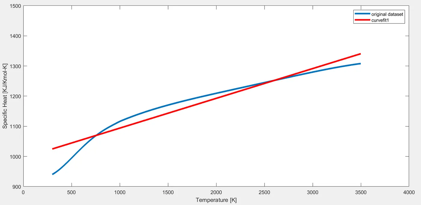
co_effs1 = polyfit(temperature,cp,1); %polyfit command to estimate the co-efficients a,b,c
predicted_cp = polyval(co_effs1,temperature);% ployval command to calculate the predicted Cp

%plotting to compare linear polynomial curvefit with the original data
plot(temperature,cp,'linewidth',3); % plotting curve for given original data
hold on
plot(temperature,predicted_cp,'linewidth',3,'color','r')% plotting curve for linear polynomial predicted data

xlabel('Temperature [K]') %labelling x-axis as temperature
ylabel('Specific Heat [KJ/Kmol-K]')% labelling y-axis as specific heat(Cp)
axis([0 4000 900 1500]) %defining axis limits
legend('original dataset','curvefit1')%providing legends to curves
Plot comparing original dataset and linear polynomial curvefit.
MATLAB CODE FOR CUBIC POLYNOMIAL:
% CURVE FIT WITH CUBIC POLYNOMIAL
clear all
close all
clc

%Preparing the data
cp_data = load('data'); % loading the data from the file "data"
temperature = cp_data(:,1); % first column is temperature data
cp = cp_data(:,2);%second column is Cp data

% Curve fit
%cp = ax^3+bx^2+cx+d (cubic polynomial)
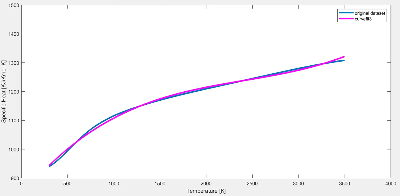
co_effs2 = polyfit(temperature,cp,3); % polyfit command to estimate the co-efficients a,b,c and d
predicted_cp1 = polyval(co_effs2,temperature);% polyvalcommand to calculate the predicted Cp

% Plotting to compare my cubic polynomial curvefit with the original data
plot(temperature,cp,'linewidth',3); % plotting curve for given original data
hold on
plot(temperature,predicted_cp1,'linewidth',3,'color','m'); % plotting curve for cubic polynomial predicted data

xlabel('Temperature [K]') %labelling x-axis as temperature
ylabel('Specific Heat [KJ/Kmol-K]')% labelling y-axis as specific heat(Cp)
axis([0 4000 900 1500]) %defining axis limits
legend('original dataset','curvefit3')%providing legends to curves
Plot comparing original dataset and cubic polynomial curvefit.
MATLAB CODE FOR LINEAR AND CUBIC POLYNOMIAL :
% CURVE FIT WITH LINEAR AND CUBIC POLYNOMIAL
clear all
close all
clc

%Preparing the data
cp_data = load('data'); % loading the data from the file "data"
temperature = cp_data(:,1); % first column is temperature data
cp = cp_data(:,2);%second column is Cp data

%%
%curve fit for linear polynomial
% cp = ax+b (linear polynomial)
co_effs1 = polyfit(temperature,cp,1); %polyfit command to estimate the co-efficients a,b,c
predicted_cp = polyval(co_effs1,temperature);% ployval command to calculate the predicted Cp

%plotting to compare linear polynomial curvefit with the original data
plot(temperature,cp,'linewidth',3); % plotting curve for given original data
hold on
plot(temperature,predicted_cp,'linewidth',3,'color','r')% plotting curve for linear polynomial predicted data

%%
% Curve fit for cubic polynomial
%cp = ax^3+bx^2+cx+d (cubic polynomial)
co_effs2 = polyfit(temperature,cp,3); % polyfit command to estimate the co-efficients a,b,c and d
predicted_cp1 = polyval(co_effs2,temperature);% polyvalcommand to calculate the predicted Cp

% Plotting to compare my cubic polynomial curvefit with the original data
plot(temperature,predicted_cp1,'linewidth',3,'color','m'); % plotting curve for cubic polynomial predicted data

%%
xlabel('Temperature [K]') %labelling x-axis as temperature
ylabel('Specific Heat [KJ/Kmol-K]')% labelling y-axis as specific heat(Cp)
axis([0 4000 900 1500]) %defining axis limits
legend('original dataset','curvefit1','curvefit3')%providing legends to curves
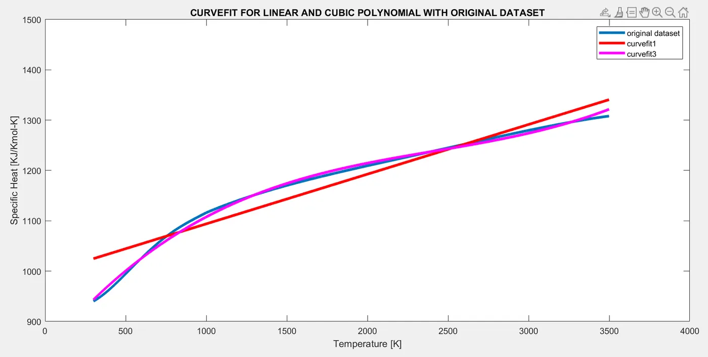
title('CURVEFIT FOR LINEAR AND CUBIC POLYNOMIAL WITH ORIGINAL DATASET')
Plot comparing original dataset , linear polynomial curvefit and cubic plonomial curvefit.
PARAMETERS USED TO MEASURE THE FITNESS CHARACTERISTICS OF CURVES:
Some parameters helps us to find the best fit for the curves.To fit a curve on the observed data is not enough.We have to measure some parameter that gives us clear understandng about the goodness of fit criteria or how well the equation is representing the data points.
Those parameters are : 1. The sum of the squares due to error(SSE)
2. R-square
3. Adjusted R-square
4 . Root mean squared error(RMSE)
How to make a curve fit perfectly?
Curvefit can be made perfect by interpolating the datasets.By interpolation the errors can be minimized and it is also possible to reduce the errors to zero. Curvefit should match with the original without showing errors.
How to get the best fit?
Line of best fit refers to a line through a scatter plot of data points that best expresses the relationship between those points.A more accurate way of finding the line of best fit is the least square method.
We can increase the order of polynomial to get the best fit.
What could be done to improve the cubic fit?
By using split-wise method we can improve a curve fit for that particular order of polynomial.By splitting the curvefits into multiple number of polynomials for different datasets of temperature and specfic heat values.
SPLIT-WISE POLYNOMIAL FUNCTION MATLAB CODE:
% split-wise curvefit
 clear all
 close all
 clc

%Extracting the data from file
cp_data = load('data'); % loading the data from the file "data"
temperature = cp_data(:,1);  % first column is temperature data
cp = cp_data(:,2); %second column is Cp data

co_efficients  = polyfit(temperature(1:1500),cp(1:1500),2); % for quadratic polynomial
co_efficients0 = polyfit(temperature(1500:3000),cp(1500:3000),3); %for cubic ploynomial

%calculating predicted specific heat values for two different sets of temperature range
predicted_cp1 = polyval(co_efficients,temperature(1:1500));
predicted_cp2 = polyval(co_efficients0,temperature(1500:3000));

%plotting graphs
plot(temperature,cp,'linewidth',3,'color','y');
hold on
plot(temperature(1:1500),predicted_cp1,'linewidth',3,'color','r');
plot(temperature(1500:3000),predicted_cp2,'linewidth',3,'color','g');
hold off

xlabel('Temperature [K]') %labelling x-axis as temperature
ylabel('Specific Heat [KJ/Kmol-K]')% labelling y-axis as specific heat(Cp)
axis([0 3500 950 1350]) %defining axis limits
legend('original dataset','linear curvefit','cubic curvefit')%providing legends to curves
title('TEMPERATURE VS Cp')
SPLIT-WISE POLYNOMIAL FUNCTION GRAPH:
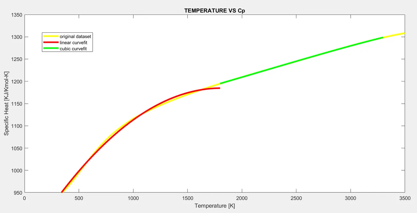
From the above graph we can observe that curvefit of cubic polynomial is more closer to the curvefit of original dataset as we use split-wise method.
REFERENCES:
https://skill-lync.com/projects/Curve-Fitting-and-criterion-to-choose-best-fit-41860
https://engineering.vanderbilt.edu/ge/es140/Otherlinks/MatlabTutorial/CurveFitting.php
http://www.math.utah.edu/~palais/pcr/spike/Evaluating%20the%20Goodness%20of%20Fit%20--%20Fitting%20Data%20(Curve%20Fitting%20Toolbox)%20copy.html