Week 3 - Solving second order ODEs

AIM: To write a program that solves the 2nd order ODE which represents the equation of motion of a simple pendulum with damping and create an animation of its motion.

OBJECTIVE :

To use this information to animation the motion of the pendulum

L=1 metre,

m=1 kg,

b=0.05.

g=9.81 m/s2.

To simulate the motion between 0-20 sec, for angular displacement=0,angular velocity=3 rad/sec at time t=0.

GOVERNING EQUATIONS:

where, b = damping co-effficient

g= gravity in m/s2,

L = length of the pendulum in m,

m = mass of the ball in kg

SIMPLE PENDULUM :

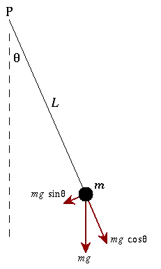
A simple pendulum consists of a mass m hanging from a string of length L and fixed at a pivot point P. When displaced to an initial angle and released, the pendulum will swing back and forth with periodic motion.Pendulum, body suspended from a fixed point so that it can swing back and forth under the influence of gravity. Pendulums are used to regulate the movement of clocks , because the interval of time for each complete oscillation, called the period is constant. The formula for the period T of a pendulum is T = 2π Square root of√^L/_g, where L is the length of the pendulum and g is the acceleration due to gravity.

MATLAB CODE:

• Firstly, the input values i.e., daming co-efficient,f=gravity,mass and length of the pendulum values are declared.
• There are 2 1st order ODE's one for velocity and one for displacement.So, the starting values of angular dispalcement is given as 0 and angular velocity is given as 3.
• We need to integrate ODE system to obtain a solution for which we need time.So,the simulation time of the motion is given between 0 - 20 sec.
• Then the ODE solver function is used to calculate the motion of the pendulum.
• ODE45 FUNCTION : The function ode45 takes three inputs.The 3 inputs are the function to be integrated,the time span and the initial conditions.
• Now to solve the second order ODE we have to break the equation such that it becomes two 1st order ODE. After that we have to create a function file which solves the equations as per our required ODE.
• Ode function with two 1st order equatons is written as a seperate function file and ode function will be called by declaring the values in the main program

function [dtheta_dt] = ode_fun(t,theta,b,g,l,m)

theta1 = theta(1)
theta2 = theta(2)
dtheta1_dt = theta(2);
dtheta2_dt = -(b/m)*theta2-(g/l)*sin(theta1);
dtheta_dt = [dtheta1_dt; dtheta2_dt];

end

• The plot between velocity vs time and displacement vs time will be obtained.
• By giving the values for line length and mass of the bob values the plot for simple pendulum motion will be obtained.
• Then the animation for the motion of the pendulum can be done by using Movie command.

clear all 
close all 
clc

b = 0.8;  %damping co-efficient 
g = 9.81; % gravity
L = 1;    % length of the pendulum
m = 1;    % mass of the bob

%initial condition 
theta_0 = [0;3];

%time points
t_span = linspace(0,20,500);

%solve ODE
[t,results] = ode45(@(t,theta) ode_fun(t,theta,b,g,L,m),t_span,theta_0);

%plotting 
figure(1),clf
plot(t,results(:,1),'linewidth',3,'color','g');
hold on
plot(t,results(:,2),'linewidth',3,'color','r');
legend('time vs displacement','time vs velocity');
xlabel('time')
ylabel('angular-velocity & angular-displacement')

% creating an animation of a simple pendulum
%initial point or fixed point
x0 = 0;
y0 = 0;
    
ct = 1;
for i = 1:length(t)
    %calculation of second point
    x1 = L*sin(results(i,1));
    y1 = -(L*cos(results(i,1)));
    figure(2),clf
    hold on
    plot([-L-0.5 L+0.5],[0,0],'linewidth',2,'color','k')
    plot([0 0],[-5 5],'k--','linewidth',1)
    plot([x0,x1],[y0,y1],'k','linewidth',2)
    plot(x1,y1,'o','markerfacecolor','m','markersize',30,'markeredgecolor','r')
    axis([-L-1,L+1,-L-2,0.5])
    axis off
    title('ANIMATION OF SIMPLE PENDULUM')
    grid on
    M(ct) = getframe(gcf);
    ct = ct+1;
end

% Creating a movie
movie(M)
videofile = VideoWriter('PENDULUM.avi','Uncompressed AVI');
open(videofile)
writeVideo(videofile,M)
close(videofile)

RESULTS:

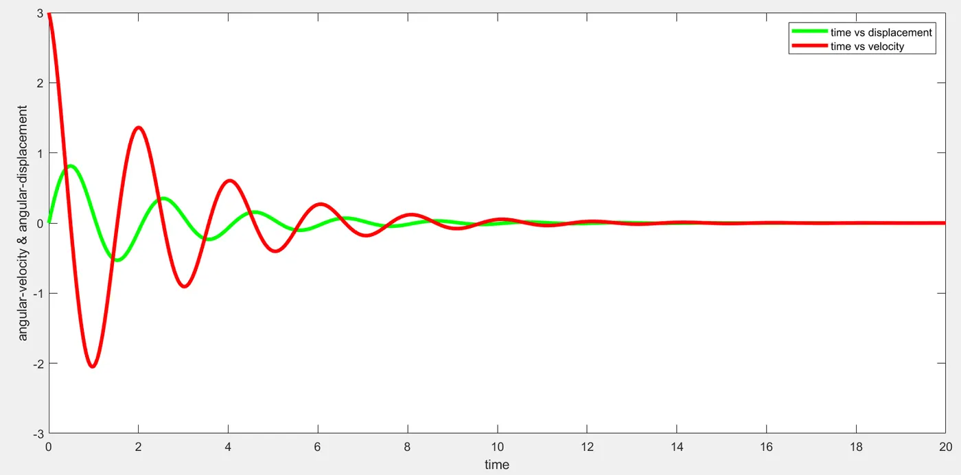
The plot for angular-velocity and angular-displacement w.r.t time

ANIMATION OF SIMPLE PENDULUM:

YOUTUBE VIDEO LINK:

https://youtu.be/sCoYyzmaU84

ERRORS:

In animation code , I have written Uncompressed.AVI because of that mistake MATLAB did not display animation video.

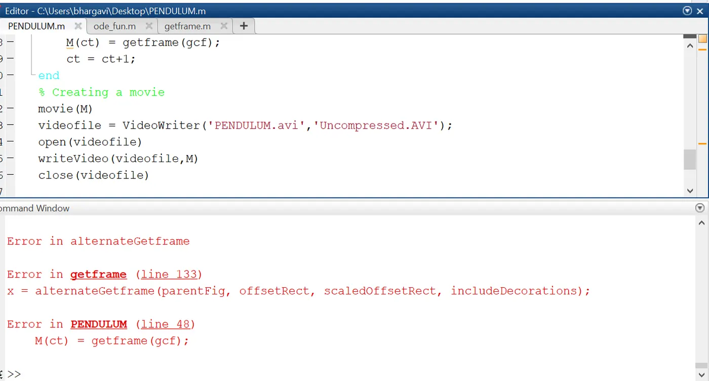
After removing dot i.e., writing Uncompressed.AVI animation is displayed.

CONCLUSION:

By ODE function the equation of the motion of simple pendulum is solved and animation of the pendulum is obtained.