Week 4 - Genetic Algorithm

AIM : To write a MATLAB code for optimisation of stalagmite function using genetic algorithm.

OBJECTIVE : 1. To find the global maxima of the function

2. To obtain a single solution for the function irrespective of number of executions.

GOVERNING EQUATIONS :

`f_(1,x) = [sin(5.1*pi*x +0.5)]^6`

`f_(1,y) = [sin(5.1*pi*y + 0.5)]^6`

`f_(2,x) = exp(-4 * ln(2)* (x - 0.0667)^2/0.64)`

`f_(2,y) = exp(-4*ln(2)*(y-0.0667)^2/0.64)`

STALAGMITE :

A stalagmite is an upward-growing mound of mineral deposits that have precipitated from water dripping onto the floor of a cave. Most stalagmites have rounded or flattened tips.Stalagmites grow from the cave floor.Stalagmite and stalactite functions are mathematical functions which represent shapes similar to the stalagmite and stalactite structures.

GENETIC ALGORITHM :

The genetic algorithm is a method for solving both constrained and unconstrained optimization problems that is based on natural selection, the process that drives biological evolution. The genetic algorithm repeatedly modifies a population of individual solutions. At each step, the genetic algorithm selects individuals at random from the current population to be parents and uses them to produce the children for the next generation.

Over successive generations, the population "evolves" toward an optimal solution. You can apply the genetic algorithm to solve a variety of optimization problems that are not well suited for standard optimization algorithms, including problems in which the objective function is discontinuous, nondifferentiable, stochastic, or highly nonlinear. The genetic algorithm can address problems of mixed integer programming, where some components are restricted to be integer-valued.

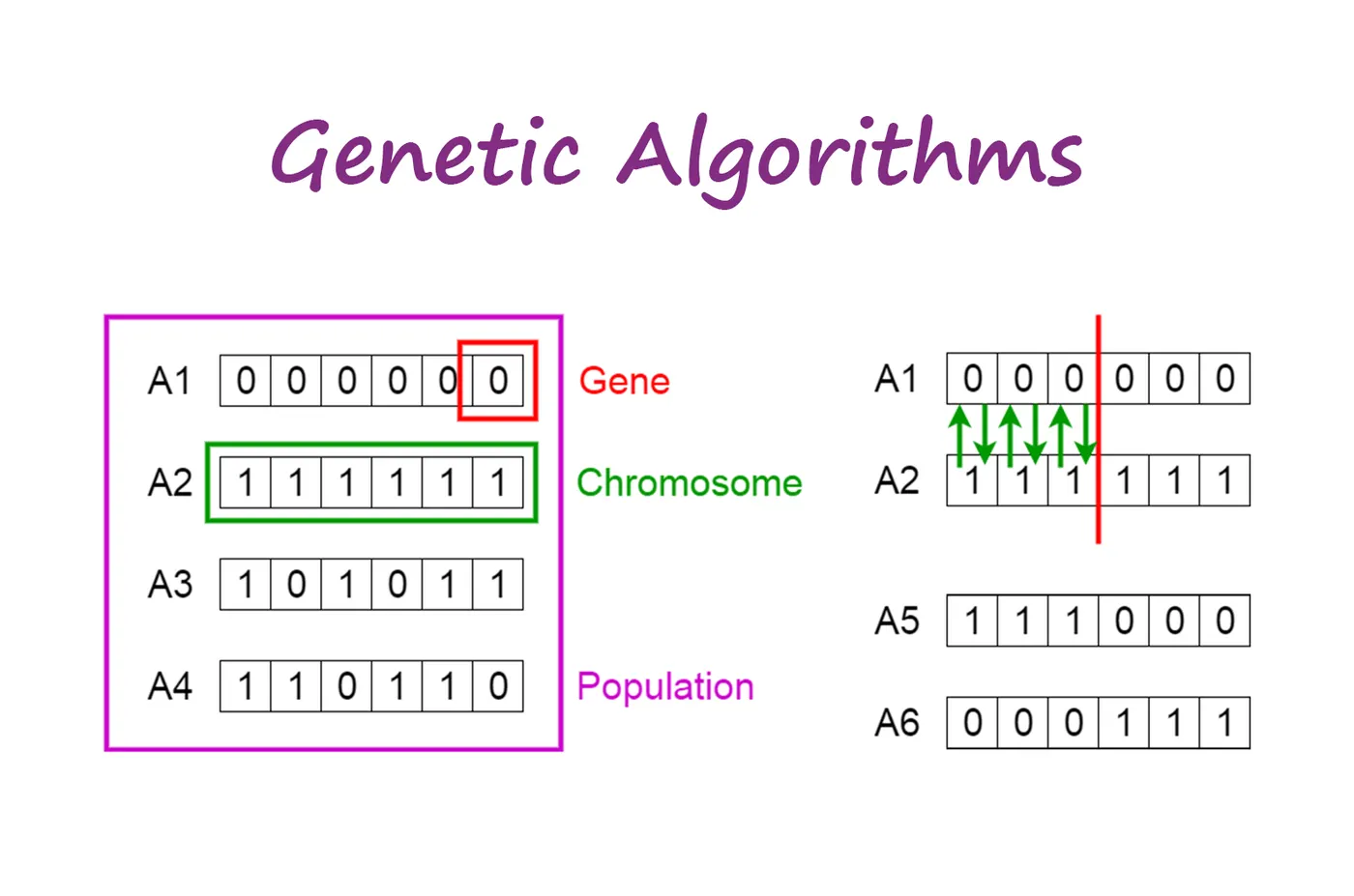
NOTION OF NATURAL SELECTION :

The process of natural selection starts with the selection of fittest individuals from a population. They produce offspring which inherit the characteristics of the parents and will be added to the next generation. If parents have better fitness, their offspring will be better than parents and have a better chance at surviving. This process keeps on iterating and at the end, a generation with the fittest individuals will be found.

This notion can be applied for a search problem. We consider a set of solutions for a problem and select the set of best ones out of them.

Five phases are considered in a genetic algorithm.

1. Initial population
2. Fitness function
3. Selection
4. Crossover
5. Mutation

INITIAL POPULATION :

The process begins with a set of individuals which is called a Population. Each individual is a solution to the problem we want to solve.

An individual is characterized by a set of parameters (variables) known as Genes. Genes are joined into a string to form a Chromosome (solution).

In a genetic algorithm, the set of genes of an individual is represented using a string, in terms of an alphabet. Usually, binary values are used (string of 1s and 0s). We say that we encode the genes in a chromosome.

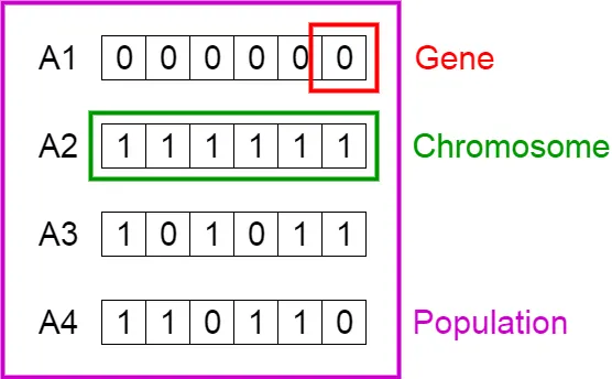
Population, Chromosomes and Genes

FITNESS FUNCTION:

The fitness function determines how fit an individual is (the ability of an individual to compete with other individuals). It gives a fitness score to each individual.

The probability that an individual will be selected for reproduction is based on its fitness score.

SELECTION :

The idea of selection phase is to select the fittest individuals and let them pass their genes to the next generation.

Two pairs of individuals (parents) are selected based on their fitness scores. Individuals with high fitness have more chance to be selected for reproduction.

CROSSOVER :

Crossover is the most significant phase in a genetic algorithm. For each pair of parents to be mated, a crossover point is chosen at random from within the genes.

For example, consider the crossover point to be 3 as shown below.

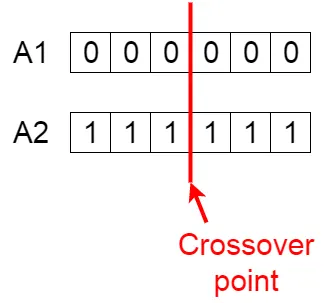
Crossover point

Offspring are created by exchanging the genes of parents among themselves until the crossover point is reached.

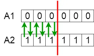
Exchanging genes among parents

The new offspring are added to the population.

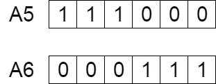
New offspring

MUTATION :

In certain new offspring formed, some of their genes can be subjected to a mutation with a low random probability.

This implies that some of the bits in the bit string can be flipped.

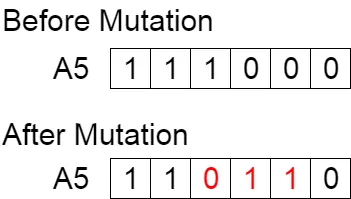
Mutation: Before and After

Mutation occurs to maintain diversity within the population and prevent premature convergence.

TERMINATION :

The algorithm terminates if the population has converged (does not produce offspring which are significantly different from the previous generation). Then it is said that the genetic algorithm has provided a set of solutions to our problem.

SYNTAX FOR GENETIC ALGORITHM :

In matlab,genetic algorithm runs using a solver name 'ga'.In matlab genetic algorithm gives the minimum value of the function.It always tries to minimise the given fitness function.But, it can also be used to both minimum or maximum value of the function.

Syntax for ga : [Input,fval] = ga(func,nvars,A,b,Aeq,Beq,lb,ub,nonlcon,Intcon,options)

Input - returns the input values

fval - returns the vaalues of the fitness function.

ga - Solver inbuilt in matlab

func - function which we desires to minimize

nvars - No. of variables associated with the function

A and b - Matrix which represents linear inequality constraint of the type A*x`le`b (if linear inequality constraints are not mentioned then define as A = [] and b = [])

Aeq and beq - Matrix which represents equality constraints of the type A*x = b (if equality constraints are not mentioned then define as Aeq = [] and beq = [])

lb and ub - lower bound and upper bound limits for the ga.These provide the ga a search space.

nonlcon - sets non-linear constraints,if any.

Intcon - sets integer constraints, if any.

options - used whenever we want to change the default functioning of ga.

STOPPING CONDITIONS :

The genetic algorithm uses the following options to determine when to stop. See the default values for each option by running opts = optimoptions('ga').

The algorithm stops as soon as any one of these conditions is met.

CODE FOR GENETIC ALGORITHM :

clear all
close all
clc

% Defining search space
x = linspace(0,0.6,150);% Creates x 1-D array from 0 to 0.6 of 150
y = linspace(0,0.6,150);% Creates y 1-D array from 0 to 0.6 of 150
num_cases = 50; % No. of iterations for the ga function 

% Creating 2D array using meshgrid function
[xx yy] = meshgrid(x,y); % meshgrid command creates a 2-D array of above vectors

%% Evaluation of stalagmite function 
for i = 1:length(xx)
    for j = 1:length(yy)
    input_vector(1) = xx(i,j);% assigning value to the variable 
    input_vector(2) = yy(i,j); % assigning value to the variable
    F(i,j) = stalagmite(input_vector) % calling a function and giving an input to it.
    end
end

%% optimization of stalagmite function for global maxima
% study-1 statistical behaviour with unbounded inputs
tic                     % to start the stopwatch timer
thestate = rng;  % the state variable save to random stream
for i = 1:num_cases     % iterates through each number cases
   [inputs1,fval1(i)] = ga(@stalagmite,2); % assigning parameters to function 'ga'
    xopt1(i) = inputs1(1); % storing the x values
    yopt1(i) = inputs1(2); % storing the y values
end

rng(thestate); % reset the stream and rerun ga
figure(1) % to create a figure window
 subplot(2,1,1) % to create multiple figure
 hold on    % it holds the previous plot
 surfc(xx,yy,-F) % helps to create a surface contour plot
 xlabel('X-Value') % assigns name to x-axis
 ylabel('Y-Value') % assigns name to y-axis
 shading interp   % shades the surface contour
 plot3(xopt1,yopt1,fval1,'marker','o','markersize',5,'markerfacecolor','y')
 % To plot the markers on the optimum function value points
 title('Unbounded Inputs') % gives title to plot
 subplot(2,1,2)   % to create another plot on same window
 plot(fval1)
 xlabel('Iterations') %assigns name to x-axis
 ylabel('Function Maximum') %assigns name to y-axis
 study1_time = toc % end the stopwatch and assign time to given variables
  
 %% Study-2 statistical behaviour with bounded inputs
  tic              % to start the stopwatch timer
  thestate = rng; % the state variable save to random stream
  for i = 1:num_cases     % helps to allocate the upper and lower bound to ga
      [inputs2,fval2(i)] = ga(@stalagmite,2,[],[],[],[],[0;0],[0.6;0.6]); %assigning variables to function ga
      xopt2(i) = inputs2(1); %assigning variables to output obtained
      yopt2(i) = inputs2(2); %assigning variables to output obtained
  end
   rng(thestate); % end the stopwatch and assign the time to given variables
    figure(2)         % to create a figure window
    subplot(2,1,1)    % to create multiple figure 
    hold on           % it holds the previous plot
    surfc(xx,yy,-F)    % helps to create a surface contour plot
    xlabel('X-value') % assigns names to x-axis 
    ylabel('Y-value') % assigns names to y-axis
    shading interp    % shades the surface contour
    % to plot the markers on the optimum function value points
    plot3(xopt2,yopt2,fval2,'marker','o','markersize',5,'markerfacecolor','g')
    title('BOUNDED INPUTS') %gives title to plot
    subplot(2,1,2)           % to create another plot on same window 
    plot(fval2)
    xlabel('Iterations')     % assigns name to x-axis
    ylabel('Function maximum') %assigns name to y-axis
    study2_time = toc % end the stopwatch and assign time to given variables
    
   %% Study-3 Increasing population size 
   options = optimoptions('ga','populationsize',180) %giving parameters to ga
   tic
   thestate = rng;  % increases the population size
   for i = 1:num_cases
       [inputs3,fval3(i)] = ga(@stalagmite,2,[],[],[],[],[0;0],[0.6;0.6],[],[],options);
       xopt3(i) = inputs3(1); % storing the xvalues
       yopt3(i) = inputs3(2); % storing the y values
   end
   rng(thestate);
   figure(3) % to create figure window
   subplot(2,1,1) % to create multiple figure
   hold on         % it holds the previous plot
   surfc(xx,yy,-F) % helps to create a surface contour plot
   xlabel('X-value') % assigns names to x-axis
   ylabel('Y-value') % asssigns names to y-axis
   shading interp    %shades the surace contour
   plot3(xopt3,yopt3,fval3,'marker','o','markersize',5,'markerfacecolor','b')
   title('BOUNDED INPUTS WITH GIVEN POPULATION SIZE')
   subplot(2,1,2)  % to create another plot on same window
   plot(fval3)     
   xlabel('Iterations') %assigns names to x-axis
   ylabel('Function maximum')% asssigns names to y-axis
   study3_time = toc %end the stopwatch 
   
   %% To find maxima at a iteration 
   [Max Ival] = max(abs(fval3))
   % max function helps to find the maximum value of fval and the corresponding 
   iteration(Ival).
   
  
 
    

CODE FOR STALAGMITE ALGORITHM :

function[F] = stalagmite(input_vector)
x1 = input_vector(1);
y1 = input_vector(2);

f1_x = [sin(5.1*pi*x1+0.5)].^6;
f1_y = [sin(5.1*pi*y1+0.5)].^6;
f2_x = exp(-4*log(2).*((x1-0.0667).^2/0.64));
f2_y = exp(-4*log(2).*((y1-0.0667).^2/0.64));

F = -(f1_x.*f2_x.*f1_y.*f2_y);

EXPLANATION :

Firstly, a random array of x and y values were created and the corresponding 2D array was created using meshgrid function.

MESHGRID :[X,Y] = meshgrid(x,y) transforms the domain specified by vectors x and y into arrays X and Y, which can be used to evaluate functions of two variables and three-dimensional mesh/surface plots.

A nested loop was used to assign values from 2D array into an input_vector array.

Tic and toc commands are used to get the running time of each study.

In study-1 bounds are not defined and plots were made.

In study-2 bounds are defined and plot obtained is more accurate.

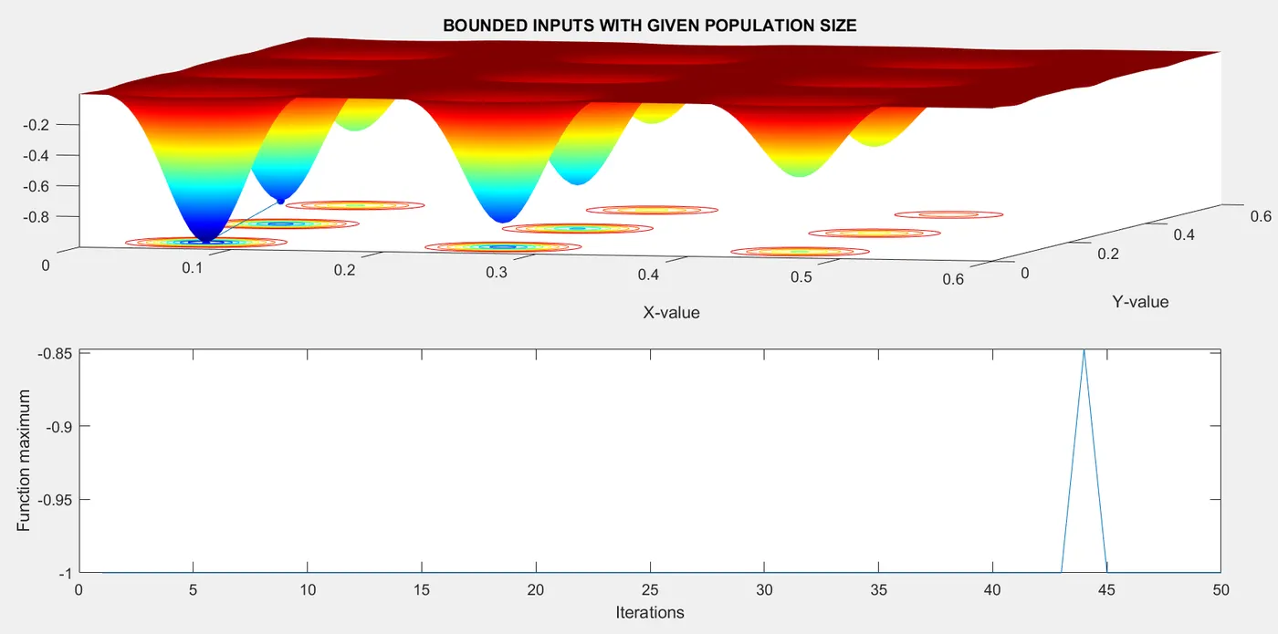
In study - 3 the population size is increased and plotting is done. Global maxima is found in this study.

Negative sign is given to the stalagmite function output F inside surface function to get the output graph upwards.

The iterations were decreased to such a value that results do not vary.

RESULTS :

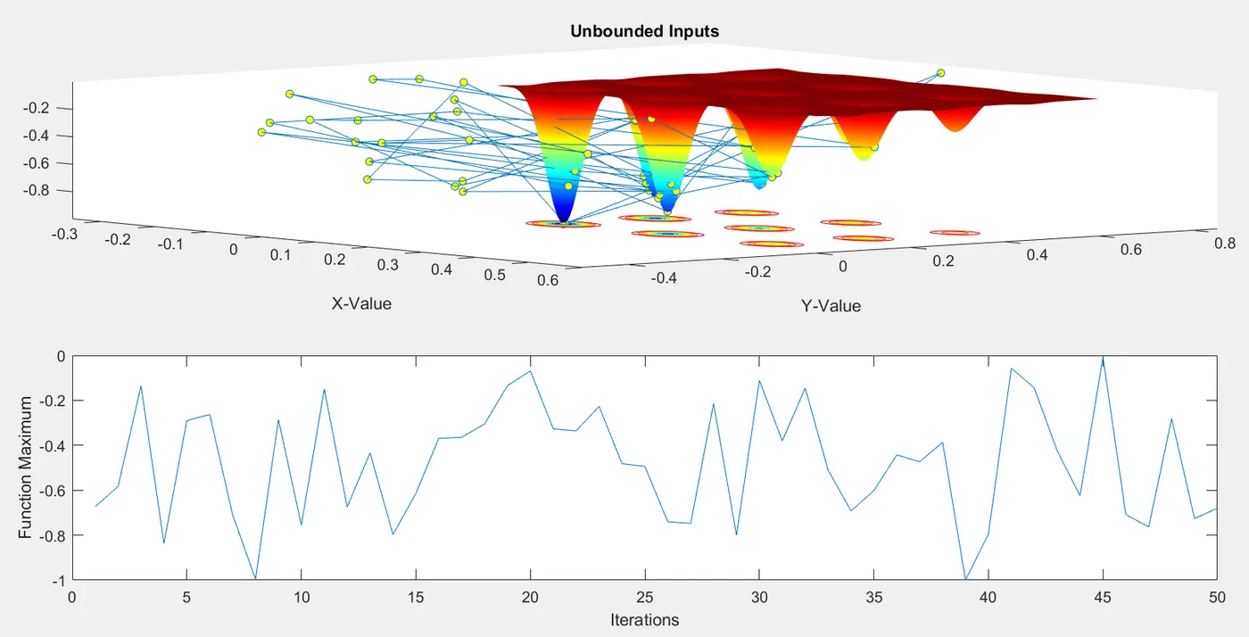
STUDY -1 :

Here no constraints and options are defined.So the graph is ireggular and many maxima points are obtained.Study required is less due to no constraints.

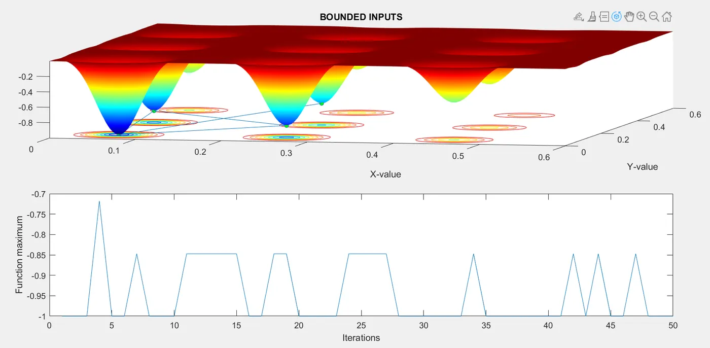
STUDY - 2

In this case bounds are defined and we could see a much better plot.All the points are confined to much closer space.

STUDY - 3:

The time required for this plot compared to other cases.Setting the population size helped to obtain local and global maxima.

Conclusion :

1. We learnt about the optimisation of a function and understood the working of genetic algorithm in matlab.

2. As we increase the number of iterations we will get the clear idea of genetic algorithm functionality and hence helps in obtaining local and global maxima.

REFERENCES:

https://www.analyticsvidhya.com/blog/2017/07/introduction-to-genetic-algorithm/

https://www.mathworks.com/help/gads/how-the-genetic-algorithm-works.html#f6243

https://www.tutorialspoint.com/genetic_algorithms/genetic_algorithms_survivor_selection.htm

https://www.mathworks.com/help/gads/options-in-genetic-algorithm.html