Curve Fit Using Matlab

AIM

To write a program to best fit the curve for Specific Heat and Temparature

OBJECTIVES

1) To Load the file into Matlab

2) To store Temperature and Specific Heat into seperate variable

3) To find Co-effecients for the equations

4) To find the predicted Polynomial values and compare it with actual values

5) To find the R Square value to determine the perfectness

6) To Compare the Predicted curve and actual curve

7) To Compare the resut from Curve fitting ToolBox with our Predicted values

FORMULAS & DEFINITIONS

1) Quadratic Equation

ax²+bx+c=0

Where,

a≠0 (If a=0, Then equation Becames bx+c=0 Which is of linear in Nature)

2) SST

The sum of squares total (SST), is the squared differences between the observed dependent variable and its mean. It is a measure of the total variability of the dataset.

SST=SSR+SSE

3) SSR

Sum of squares due to regression (SSR), is the sum of the differences between the predicted value and the mean of the dependent variable. If this value of SSR is equal to the sum of squares total, it means our regression model captures all the observed variability and is perfect

4) SSE

Sum of squares error (SSE) is the difference between the observed value and the predicted value.

5) R Square

r_square=SSR/(SSR+SSE)

• It is a relative measure and takes values ranging from 0 to 1. An R-squared of zero means our regression line explains none of the variability of the data.
• An R-squared of 1 would mean our model explains the entire variability of the data.
• Unfortunately, regressions explaining the entire variability are rare. What we usually observe are values ranging from 0.2 to 0.9.

PROGRAM

Program with 3rd polynomial order

clear all
close all
clc

cp_data = load ('data'); %LOADED DATA FILE INTO CP_DATA VARIABLE
temperature = cp_data(:,1);  %LOADED FIRST COLUMN OF CP_DATA INTO TEMPERATURE
cp=cp_data(:,2);   %LOADED SECOND COLUMN OF CP_DATA INTO TEMPERATURE


%curve fit
%cp = a*T^2+b*T+c
co_eff=polyfit(temperature,cp,3); %CALLED OUT POLYFIT TO FIND & STORE VARIABLES A,B,C UNDER CO_EFF
predicted_cp = polyval(co_eff, temperature); %STORED POLYNOMIAL VALUES W.R.T. TEMPERATURE IN PREDICTED_CP

SSR=0; %DEFINING SSR TO BE 0 AT FIRST
SSE=0; %DEFINING SSE TO BE 0 AT FIRST
mean=sum(cp)/3200; %FINDING THE MEAN

for i=1:length(cp) %LOOP WILL RUN FOR THE LENGTH OF CP
    
    SSR=SSR+(predicted_cp(i)-mean)^2; %SUMMATION OF SSR FOR EACH VALUE OF CP
    SSE=SSE+(predicted_cp(i)-cp(i))^2; %SUMMATION OF SSE FOR EACH VALUE OF CP

end

r_square=SSR/(SSR+SSE) %FINDING R_SQUARE FOR CALCULATING EFFECIENCY

%plotting
plot(temperature,cp,'linewidth',1,'color','r')
xlabel('Temperature [K]','color','r')
ylabel('Specific Heat [KJ/Kmol-K]','color','r')

hold on
plot(temperature,predicted_cp,'linewidth',3,'color','b')
legend('Specific Heat','Predicted Specific Heat')

OUTPUT

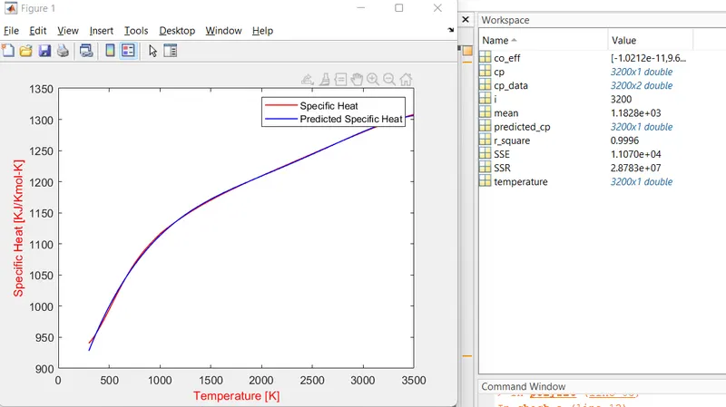
We have got an output with R² value as 0.9996 Close to 1

ERROR/WARNINGS IN THE PROGRAMS

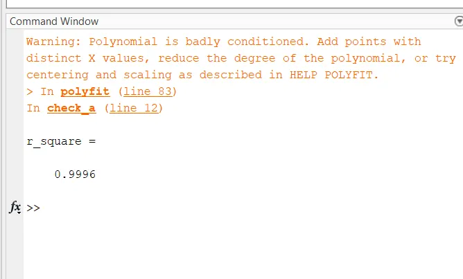
Polynomial of the code is badly constrained as there is no need for higher order, This could be eliminated by SPLIT WISE METHOD.

SPLIT WISE METHOD

clear all
close all
clc

cp_data = load ('data'); %LOADED DATA FILE INTO CP_DATA VARIABLE
temperature = cp_data(:,1);  %LOADED FIRST COLUMN OF CP_DATA INTO TEMPERATURE
cp=cp_data(:,2);   %LOADED SECOND COLUMN OF CP_DATA INTO TEMPERATURE

%splitting up the values into 3 sets
temperature_1=temperature(1:1000);
temperature_2=temperature(1001:2000);
temperature_3=temperature(2001:3200);
cp_1=cp(1:1000);
cp_2=cp(1001:2000);
cp_3=cp(2001:3200);

%curve fit
%cp = a*T^2+b*T+c
co_eff_1=polyfit(temperature_1,cp_1,3); %CALLED OUT POLYFIT TO FIND & STORE VARIABLES A,B,C UNDER CO_EFF
predicted_cp_1 = polyval(co_eff_1, temperature_1); %STORED POLYNOMIAL VALUES W.R.T. TEMPERATURE IN PREDICTED_CP

SSR=0; %DEFINING SSR TO BE 0 AT FIRST
SSE=0; %DEFINING SSE TO BE 0 AT FIRST
mean=sum(cp)/3200; %FINDING THE MEAN

%R_SQUARE FOR FIRST 1000 VALUES
for i=1:length(cp_1) %LOOP WILL RUN FOR THE LENGTH OF CP
    
    SSR=SSR+(predicted_cp_1(i)-mean)^2; %SUMMATION OF SSR FOR EACH VALUE OF CP
    SSE=SSE+(predicted_cp_1(i)-cp_1(i))^2; %SUMMATION OF SSE FOR EACH VALUE OF CP

end

r_square_1=SSR/(SSR+SSE) %FINDING R_SQUARE FOR CALCULATING EFFECIENCY

%R_SQUARE FOR SECOND 1000 VALUES
co_eff_2=polyfit(temperature_2,cp_2,3); 
predicted_cp_2 = polyval(co_eff_2, temperature_2); 

for i=1:length(cp_2) 
    
    SSR=SSR+(predicted_cp_2(i)-mean)^2;
    SSE=SSE+(predicted_cp_2(i)-cp_2(i))^2;

end

r_square_2=SSR/(SSR+SSE) 

%R_SQYARE FOR LAST 1200 VALUES
co_eff_3=polyfit(temperature_3,cp_3,2); 
predicted_cp_3 = polyval(co_eff_3, temperature_3);

for i=1:length(cp_3)
    
    SSR=SSR+(predicted_cp_3(i)-mean)^2;
    SSE=SSE+(predicted_cp_3(i)-cp_3(i))^2;

end
r_square_3=SSR/(SSR+SSE);

%Summation of 3 dataset Outputs
r_square=(r_square_1+r_square_2+r_square_3)/3; %MEAN OF R_SQUARE
predicted_cp_total=[predicted_cp_1;predicted_cp_2;predicted_cp_3];
total_temperature=[temperature_1;temperature_2;temperature_3];

%plotting
plot(temperature,cp,'linewidth',1,'color','r')
xlabel('Temperature [K]','color','r')
ylabel('Specific Heat [KJ/Kmol-K]','color','r')

hold on

plot(total_temperature,predicted_cp_total,'linewidth',1,'color','b')
legend('Specific Heat','Predicted Specific Heat')

OUTPUT OF SPLIT WISE METHOD

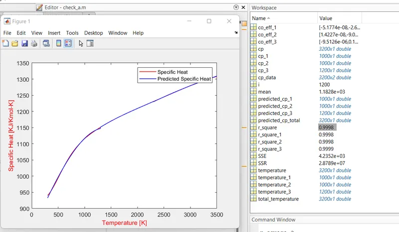
In this method the R value is increased by 0.0002

Curve fitting ToolBox

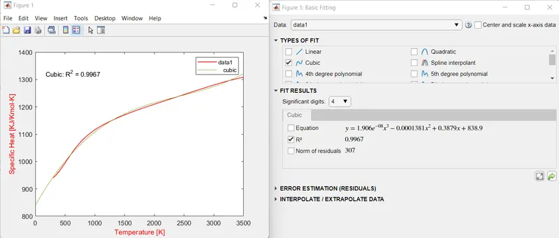
Once the figure window appears go to Tools and then click on Basic Fitting. Basic Fitting Window appears.

From the Cubic Polynomial, It's evident that the R square value Matches with our Code.

Conclusion

Hence it's verified that the R square value could be increased by Split wise Method and also the Basic Fitting matches with our code