PV Diagram of a Otto cycle Using Matlab

Aim

Write a program to visualize PV diagram and to then to calculate the Thermal efficiency of air standard cycle.

Objectives

1) To define the Atmospheric Pressure, Temperature & Specific heat capacity of air (Gamma).

2) To define the ignition temperature at state 3.

3) To define Bore diameter, Stroke length, Compression Ratio and Connecting rod length.

4) To calculate swept volume and clearance volume

5) To calculate Volume at state 1 and state 2 using Clearance volume and swept volume

6) To find Pressure and temperature at stage 2 Combined Gas Law

7) To calculate a Pressure at Stage 3 using Gay-Lussac's Law

8) To calculate a Pressure, Temperature & Volume of Stage 4 using Combined Gas Law and Gay-Lussac's Law

9) To trace a Curve for Compression stroke and expansion stroke using Engine Kinematics

10) To calculate the Thermal Efficiency and to plot the results

Formulas & Definitions

1) Specific Heat Capacity / Heat Capacity ratio

Specific heat capacity is the ratio of heat capacity at constant pressure to the heat capacity at constant volume

γ=Cp/Cv %For air Specific Heat Capacity is 1.4

2) Compression Ratio

The compression ratio is the ratio between the volume of the cylinder and combustion chamber in an internal combustion engine at their maximum and minimum values.

Compression Ratio=Total Volume/Clearance Volume

3) Total Volume

Total Volume is the summation of Clearance volume and Swept Volume

Total Volume=Clearance volume + Swept Volume

4) Clearance volume

Clearance Volume is the volume remaining after a Piston is positioned at Top Dead Center (TDC)

5) Swept Volume

Swept Volume is the Volume covered between Top Dead Center (TDC) and Bottom Dead Center (BDC)

6) Boyle’s law

The volume of a gas is inversely proportional to the pressure when temperature and amount of substance is constant.

P1V1 = P2V2

7) Charle’s law

The volume of a gas is directly proportional to the temperature when pressure and amount of substance is constant

V1/T1 = V2/T2

8) Combined Gas Law

Using Charle's law & Boyle’s law, We can formulate Combined Gas Law as follows

P1V1/T1 = P2V2/T2

9) Formula for Tracing a curve using Engine Kinematics

V/Vc=1+1/2(Rc-1)R+1-Cos Θ-(R^2-Sin^2 Θ)^(1/2)

Where,

Rc = Compression Ratio

R = Connecting Rod Length/Crank end Radius

10) Thermal Efficiency

The thermal efficiency of a heat engine is the percentage of heat energy that is transformed into work.

Thermal Efficiency = 1-(QOUT/QIN)

Where

QOUT = t4-t1

QIN = t3-t2

Program

clear all
close all
clc

%inputs
gamma=1.4 %Ratio of Specific Heat for air
t3=2300 %Temperature at an ignition state

%state variables
p1=101325 %atmospheric pressure
t1=500 %atmospheric Temperature

%engine geomentric parameters
bore=0.1 %bore dia
stroke=0.1 % stroke length
con_rod=0.15 %connecting rod length
cr=12 %compression ratio

%calculating swept vol & clearance vol

v_swept=(pi/4).*bore.^2*stroke %swept volume
v_clearance=v_swept/(cr-1) %clearance volume
v1=v_clearance+v_swept %volume at state 1
v2=v_clearance %volume at state 2

%state variables at state points 2
%p2v2^gamma=p1v1^gamma
%p2=p1*(v1/v2)^gamma=p1*cr^gamma

p2=p1*cr^gamma %pressure at state 2

%p1v1/t1=p2v2/t2 | t2=p2v2t1/(p1v1)
t2=p2*v2*t1/(p1*v1) %temperature at state 2

constant_c = p1*v1^gamma %defining a constant for compression stroke
V_compression = engine_kinematics(bore,stroke,con_rod,cr,180,0) %calling function for tracing curve for volumentric compression using engine Kinematics
P_compression = constant_c./V_compression.^gamma; %tracing curve for pressure in compression stage using engine Kinematics

%state variables at state points 3
v3=v2 %since Constant volume heat addition

%p3v3/t3=p2v2/t2 | p3=p2*t3/t2
p3=p2*t3/t2  %calculating the pressure after ignition



constant_c = p3*v3^gamma %defining a constant for expansion stroke
V_expansion = engine_kinematics(bore,stroke,con_rod,cr,0,180) %calling function for tracing curve for volumentric expansion using engine Kinematics
P_expansion = constant_c./V_expansion.^gamma; %tracing curve for pressure in compression stage using engine Kinematics



%%state variables at state points 4
v4=v1 %constant volume heat rejection process

%p3v3^gamma=p4v4^gamma | p4=p3(v3/v4)^gamma
p4=p3*(v3/v4)^gamma %calculating the pressure after heat rejection

t4 = p4*v4*t3/(p3*v3); %temperature at state 4

%thermal Effeciency
QOUT = t4-t1; %Work out
QIN = t3-t2;  %Work input
thermal_effeciency = 1-(QOUT/QIN); %thermal Effeciency



figure(1)
hold on
plot(v1,p1,'*','color','r')
plot(V_compression,P_compression,'color','r')
plot(v2,p2,'*','color','r')
plot([v2 v3],[p2 p3],'color','r')
plot(v3,p3,'*','color','r')
plot(V_expansion,P_expansion,'color','b')
plot([v4 v1],[p4 p1],'color','b')
plot(v4,p4,'*','color','b')
xlabel('VOLUME','color','b')
ylabel('PRESSURE','color','b')

Functions Called out in the Code

function[V] = engine_kinematics(bore,stroke,con_rod,cr,start_crank,end_crank)
a=stroke/2;
R=con_rod/a;

%calculating swept vol & clearance vol

v_s=(pi/4)*bore.^2*stroke;
v_c=v_s/(cr-1);

theta=linspace(start_crank,end_crank,100);


term1=0.5*(cr-1);
term2=R+1-cosd(theta);
term3=(R.^2-sind(theta).^2).^0.5;
V=(1+term1*(term2-term3)).*v_c;


end

Output of the code

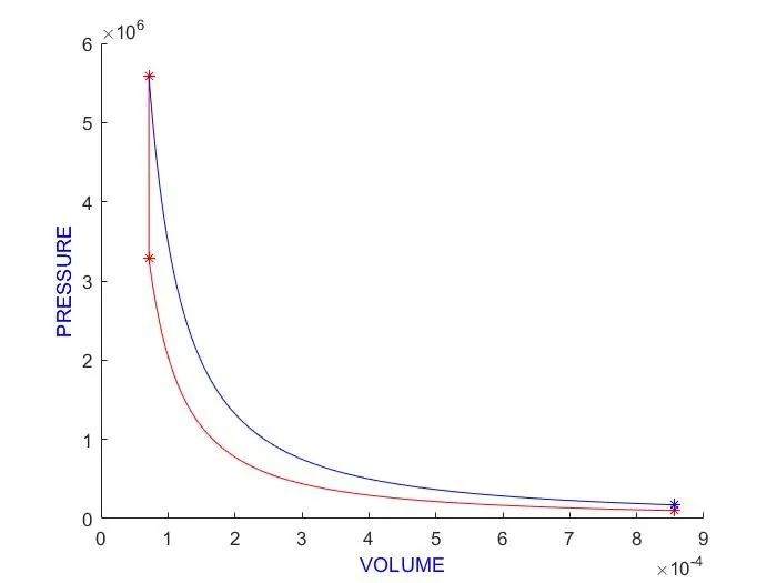
PV Diagram of the Air Standard Cycle

Thermal Efficiency

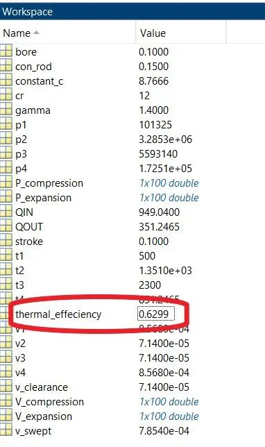
Result

Hence the PV Diagram was plotted and Thermal Efficiency was found out Sucessfully.