Genetic Algorithm Using Matlab

Aim

To write a code in Matlab to optimise the given function to find the Global Maxima of the function

Objectives

1) To form meshgrid using X & Y values.

2) To create a seperate function for feeding in GA.

3) To define a variable for storing an integer, the integer would be called in Loop for running the GA no. of times.

4) Study 1 depicts GA optimised by running for the particular number of times, and also to calculate the study time

5) Study 2 bounds were defined and made the GA to look into it.

6) In study 3 bounds as well as the Population size of GA were optimised to get the more accurate values

Definitions

In general optimization is the process of making the best or most effective use of a situation or resource. There were 2 main methods of optimization

1) Deterministic Method

2) Stochastic Method

1) Deterministic Method

In this approach the solver moves from one solution to another by using set of rules, Meaning the results were more rigid in nature. Example - Calculating the Volts needed for the motor to run at a particular speed.

2) Stochastic Method

In this approach there were lots of factors to be considered, Hence the results we get using this method may vary in a large scale.

Example - Population Growth in a country, Weather Prediction, Techtonic Plate Movements, Etc..,

Genetic Algorithm(GA)

Genetic algorithm is a based on natural selection theory by Charle's Darwin, where the fittest individuals are selected for reproduction in order to produce offspring of the next generation.

A genetic algorithm works by building a population of chromosomes which is a set of possible solutions to the optimization problem. Within a generation of a population, the chromosomes are randomly altered in hopes of creating new chromosomes that have better evaluation scores.

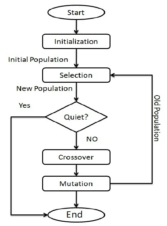
Above Flow Chart best illustrates the flow of Genetic Algorithm process.

Variable

Parameters, which will be varied during the optimization process

Constraints

Limit beyond which the GA should't search.

Variable Bound

Range of input variable, which will be varied for every iteration to provide an optimised result

Objective Function

A Simple Mathematical formulae to predict mathematical model to include all variables as input.

Genetic Algorith Syntax & Explanation

x = ga(fun,nvars,A,b,Aeq,beq,lb,ub,nonlcon,intcon,options)

Where,

fun = Seperate function to be called

nvar = Number of Variables

A & b = Linear Inequality Constraints

Aeq & beq = Linear Equality Constraints

lb = Lower Bounds

ub = Upper Bounds

nonlcon = Non Linear Constraints

intcon = Integer Variables

Options = Optimization Options

CODE & EXPLANATION

In the first study case we will see interpret Genetic Algorithm, without altering Bounds or Population Size.

First step is of the program is to define x & y values, and pass it into Stalagmite function using Nested For Loop to ensure for each value of x, the y should be passed through the loop. Once the values are passed into the Stalagmite Function, then the output of the function will be stored seperately.

clear all
close all
clc

%defining search page
x=linspace(0,0.6,150);
y=linspace(0,0.6,150);
[xx,yy]=meshgrid(x,y);
num_cases=50;

for i=1:length(x)
    for j=1:length(y)
        input_vector(1)=xx(i,j);
        input_vector(2)=yy(i,j);
        f(i,j)=stalagmite(input_vector);
    end
end

Support Program

Stalagmite Function Code

function [F] = stalagmite(input_vector)
x=input_vector(1);
y=input_vector(2);
f1=(sin((5.1*pi*x)+0.5))^6;
f2=(sin((5.1*pi*y)+0.5))^6;
f3=exp(-4*log(2)*(((x-0.0667)^2)/0.64));
f4=exp(-4*log(2)*(((y-0.0667)^2)/0.64));
F=-(f1*f2*f3*f4);
end

STUDY 1

Once the value of the functions were stored in the seperate variable (ie..,) 'f' in this case.

Second Step is to pass the value of 'f' into Genetic Algorithm and define the number of variables to be 2 (x & y). Then the GA returns two outputs one is x & y and the second one is to Optimised 'ga' value. For recording the consistency of the output, we are storing the values of x and y in the variables xout & yout.

tic 
for i=1:num_cases
    [inputs, fout1(i)]=ga(@stalagmite,2);
    xopt1(i)=inputs(1);
    yopt1(i)=inputs(2);
end
study_time1=toc

Also, We had used tic & toc command to analyse the time taken for the program to run the ga.

The subplot command is used in order to show the multiple graphs in the same windows, In this case the subplot command is used to display both Graphical Representation of the Global Maxima & Minima and the Line graph between Iteration Number vs ga Value.

The Plot3 command is used to create a plotting/line in 3D.

figure(1)
subplot(2,1,1)
surfc(x,y,f)
title('UNBOUNDED','Color','r')
shading interp
hold on
plot3(xopt1,yopt1,fout1,'marker','o','MarkerSize',5,'MarkerFaceColor','r')
subplot(2,1,2)
plot(fout1)
xlabel('ITERATIONS','color','r')
ylabel('Genetic Algorithm Value','color','r')

Output of Program

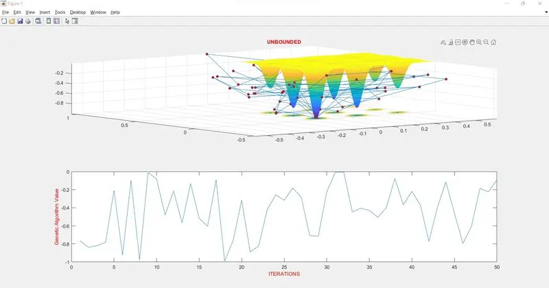
STUDY 2

In the study 2, We are defining the Lower Bounds & Upper Bounds of a 'ga' function. Rest of the things are same.

tic 
for i=1:num_cases 
    [inputs, fout(i)]=ga(@stalagmite,2,[],[],[],[],[0,0],[0.4,0.4]);
    xopt(i)=inputs(1);
    yopt(i)=inputs(2);
end
study_time1=toc

OUTPUT

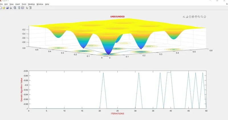
As the bounds are defined closely, we got an more accurate result.

Study 3

In the study 3 we have optimised the Population size as well as the defined bounds. 'optimoptions' is the command called optimim options, Which will be used for optimizing the predifined parameters of the solver.

options = optimoptions('ga','PopulationSize',200);
tic 
for i=1:num_cases 
    [inputs, fout3(i)]=ga(@stalagmite,2,[],[],[],[],[0,0],[0.3,0.3],[],[],options);
    xopt3(i)=inputs(1);
    yopt3(i)=inputs(2);
end

OUTPUT

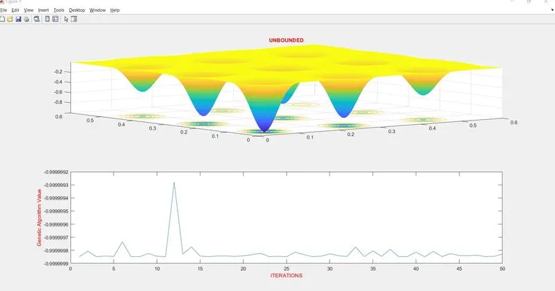
In this case the values of the ga were more streamlined in nature.

Result

Hence it's more clear that the output of the program can be more accurate in nature, by optimising the Bounds & Population size.