Creating a code to solve Otto Cycle & plot a graph betweem Pressure & volume. Calculate it’s Thermal Efficiency.
Aim-
- Creating a code to solve Otto Cycle & plot a graph bbetweem Pressure & volume.
- Calculate it’s Thermal Efficiency.
Theory-
An Otto cycle is an idealized thermodynamic cycle that describes the functioning of a typical spark ignition piston engine.
It is the thermodynamic cycle most commonly found in automobile engines.
The otto cycle help us to describe the change in mass of gas. It is depends on change in pressure temperature volume addition of heat and rejection of heat.
Objective of PROJECT:
To create a code plot a P-V diagram of otto cycle & Calculate it’s thermal Efficiency.
Process of otto cycle:
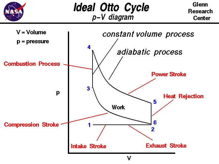
- Process 0–1 a mass of air is drawn into piston/cylinder arrangement at constant pressure.
- Process 1–2 is an adiabatic (isentropic) compression of the charge as the piston moves from bottom dead center (BDC) to top dead center (TDC).
- Process 2–3 is a constant-volume heat transfer to the working gas from an external source while the piston is at top dead center. This process is intended to represent the ignition of the fuel-air mixture and the subsequent rapid burning.
- Process 3–4 is an adiabatic (isentropic) expansion (power stroke).
- Process 4–1 completes the cycle by a constant-volume process in which heat is rejected from the air while the piston is at bottom dead center.
- Process 1–0 the mass of air is released to the atmosphere in a constant pressure process.
Equation Used In Program:
- Swept Volume
`v_(swept) = (1/2)*(b o r e)^2*stroke`
- Clearance volume
`v_(c l earance) = v_(swept)/(cr-1)`
- Compression Ratio
`cr = ((v2)/(v1))`
- Isothermal Process
`p*v^gamma = C`
- For Adiabatic Process
`(p1*v1)/(t1) = (p2*v2)/(t2)`
- Thermal Efficiency
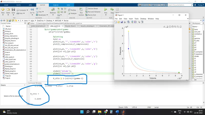
`eta_(thermal) = 1- ((v2)/(v1))^(gamma - 1)`
FUNCTION
Commands used in program
close all used for close all graph open in background
clear all used for clear all values saved in workspace
clc used for clear screen
% Used to write comment
; Used to save value in workspace but not print in command
Linspace command (Here we define only length of vector and it's interval)
Linewidth used for show thickness of line
Color command is used show different color line
Figure command used for show figure
Hold on command is used for hold multi plot in one figure
plot command is used for plot a graph between given array
grid command is used for show grid (horizontal & vertical line) in a graph
axis command is used for give a limit to axis
xlabel & ylabel command is used for write in x axis & y axis.
% INPUTS
p1, p2, p3, p4 is shown pressure at point 1,2,3&4
v1, v2, v3& v4 is shown volume at point 1,2,3,&4
t1, t2, t3& t4 is shown temperature at 1,2,3&4
Bore is diameter
stroke movement of piston from TDS to BDC
con_rod length of rod which connect crank and piston
cr for compression ratio
V_swept is swept volume
V_clearance is clearance ratio
Gamma is constant
N_otto is THERMAL EFFICIENCY
Body Of the Content
First program for plot points(figure1) and line (figure2)
% Simulating a Air Standard Cycle

clear all
close all
clc

%INPUTS
gamma = 1.4;
t3=2300;

% state variable
p1=101325;
t1=500;

%engine geometic parameters
bore=0.1;
stroke=0.1;
con_rod=0.15;       %connecting rod
cr=12;              %combustion ratio

%Calculating the swept volume and clearance volume
v_swept = (pi/4)*bore^2*stroke;
v_clearance = v_swept/(cr-1);

v1 =v_swept + v_clearance;
v2=v_clearance;

    % state variable at point2
    %p2v2^gamma=p1v1^gamma || p2=p1*(v1/v2)^gamma
    %p2=p1*(cr)^gamma
          p2=p1*(cr)^gamma;

    %p1v1/t1=p2v2/t2 || t2=p2v2*t1/p1v1
         t2=(p2*v2*t1)/(p1*v1);


    %state variable at point3
        v3=v2;
    % p3v3/t3=p2v2/t2 || p3=p2v2t3/v3t2
        p3=(p2*t3)/t2;


    %state variable at point4
        v4 = v1;
    %p3v3^gamma=p4v4^gamma
        p4=p3*(v3/v4)^gamma;

            %plotting
            hold on
            figure(1)

            plot(v1,p1,'*','LineWidth',3,'color','r')
            plot(v2,p2,'*','LineWidth',3,'color','b')
            plot(v3,p3,'*','LineWidth',3,'color','y')
            plot(v4,p4,'*','LineWidth',3,'color','g')

             xlabel('Volume');
             ylabel('Pressure');

 figure(2)
 plot([v1 v2 v3 v4 v1],[p1 p2 p3 p4 p1],'Color','b');

             xlabel('Volume');
             ylabel('Pressure');
OUTPUT:
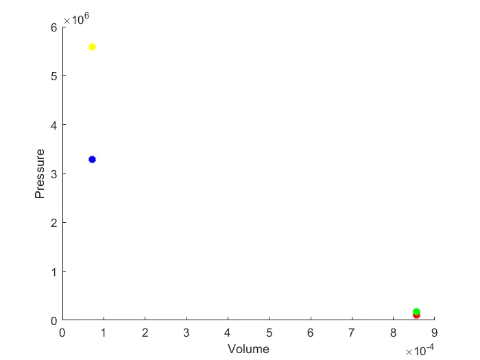
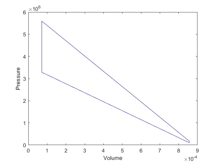
figure(1) figure(2)
Second Program:
function[V_compression]=piston_kinematics(bore,stroke,con_rod,cr,start_crank,end_crank)

a=stroke/2;
R=con_rod/a;

theta =linspace(start_crank,end_crank,100)
v_swept=(pi/4)*bore^2*stroke;
v_clearance=v_swept/(cr-1);

term1=0.5*(cr-1);
term2=R+1-cosd(theta);
term3=(R^2-sind(theta).^2).^0.5;

V_compression=(1+term1*(term2-term3)).*v_clearance
% v1=v_clearance + v_swept

end
Third Program
% Simulating a Air Standard Cycle

clear all
close all
clc

%INPUTS
gamma = 1.4;
t3=2300;

% state variable
p1=101325;
t1=500;

%engine geometic parameters
bore=0.1;
stroke=0.1;
con_rod=0.15;       %connecting rod
cr=12;              %combustion ratio

%Calculating the swept volume and clearance volume
v_swept = (pi/4)*bore^2*stroke;
v_clearance = v_swept/(cr-1);

v1 =v_swept + v_clearance;
v2=v_clearance;

    % state variable at point2
    %p2v2^gamma=p1v1^gamma || p2=p1*(v1/v2)^gamma
    %p2=p1*(cr)^gamma
          p2=p1*(cr)^gamma;

    %p1v1/t1=p2v2/t2 || t2=p2v2*t1/p1v1
         t2=(p2*v2*t1)/(p1*v1);

         constant_c=p1*v1^gamma;
         V_compression=piston_kinematics(bore,stroke,con_rod,cr,180,0);
         P_compression=constant_c./V_compression.^gamma;

    %state variable at point3
        v3=v2;
    % p3v3/t3=p2v2/t2 || p3=p2v2t3/v3t2
        p3=(p2*t3)/t2;

        constant_c=p3*v3^gamma;
        V_expansion=piston_kinematics(bore,stroke,con_rod,cr,180,0);
        P_expansion=constant_c./V_expansion.^gamma;

    %state variable at point4
        v4 = v1;
    %p3v3^gamma=p4v4^gamma
        p4=p3*(v3/v4)^gamma;

            %plotting
            hold on
            plot(v1,p1,'*','LineWidth',1,'color','r')
            plot(V_compression,P_compression)

            plot(v2,p2,'*','LineWidth',1,'color','b')
            plot([v2 v3],[p2 p3])

            plot(v3,p3,'*','LineWidth',1,'color','y')
            plot(V_expansion,P_expansion)

            plot(v4,p4,'*','LineWidth',1,'color','g')
            plot([v1 v4],[p1 p4])

            xlabel('Volume');
            ylabel('Pressure');
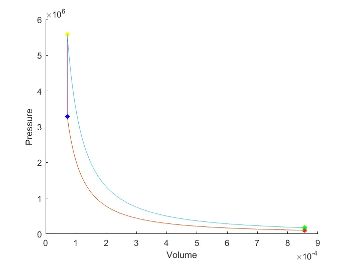
OUTPUT:
#_COMMENTS:
1. The first code describes to plot all four point of Volume-Pressure Diagram.
In this code will take inputs value of engine parameters and formula to calculate state points.
Describe adiabatic process and constant volume process.
Here we find state variable like pressure, temprature & Volume.
And plot all state point in figure(1).
2nd plot for show line which connects all the state points shown in figure (2)
2. Second program for create a function of all inputs
When two or more equation comes into a picture we can create a another program and this program is called a calling function program
In this program create a variable and a calling function.
Here we define volume by processing a engine form TDC to BDC or BDC to TDC.
For getting a no. Of values of angle theta will use linspace command
Here will use function command for run the code in first program instead of pasting code in first program.
By running this code we get different values of volume at different angle of crank.
3. Third program for create a complete PV diagram with process line.
In this code use first code and here will calling a function of second program and plot a graph.
Here function called only for plot the compression and expansion process.
And plot will generate.
# ERROR In Program
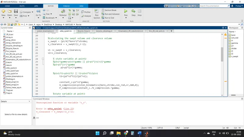
- Use different variable for compression ratio
-
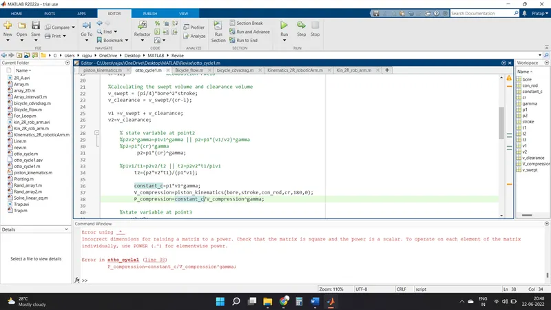
Need to use dot operator to multiple or divide array
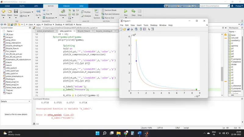
- Make error in function to show name in X axis & Y axis.
#_THERMAL EFFICIENCY:
by using Formula can get thermal efficiency:
#_NOTE:
- Calling function file name and function name should be the same.
- The first program and second program should be saved in the same folder
#_CONCLUSION:
- Various plot which generate is shown as OUTPUT of program after body of code.
BEST REGARDS
BHANU PRATAP RAJPUT