Conjugate Heat Transfer Simulation
AIM:
To simulate the Conjugate Heat Transfer analysis in cylinder pipe
Conjugate heat transfer:
Conjugate heat transfer is used to describe the processes which involves variations of temperature within the solids and fluids, due to thermal interaction between the solids and fluids.
The CHT analysis is generally used in places where there is heat transfer taking place for example when a fluid flows through a pipe and the heat of the fluid is transferred to the pipe by convection. CHT analysis is very much useful in analysing the areas where there are two bodies in which heat transfer takes place. when this analysis is used it is easy to calculate the heat transfer coefficient temperature and velocity of a fluid flowing through a certain body.
This type of heat transfer corresponds to the combination of the heat transfer in solids and heat transfer in fluids. heat transfer in solid called as conduction and heat transfer in fluid called convection.
conduction occurs due to the direct molecular collision the faster kinetic energy collides with the low speed kinetic energy and the heat transfer occur.
convection process is not happed alone. it is combined with the conduction or radiation. it occurs mostly in the cooling process like Heat sink, Battery cooling, Airflow over the solid object for cooling.
THEORY:
SUPERCYCLING:
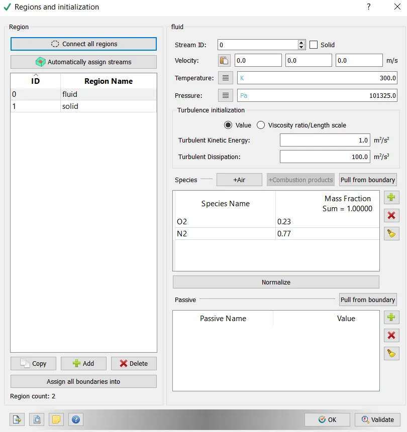
Super-cycling is a method used in converge studio for CHT problems with multiphase regions (solids and liquids). The solvers for different fluids cannot run at same speed for solving fluid it is much faster as compared to solids. If, this is done the solution does not reaches convergence. so, super cycling be used to resolve this issue. This helps solver of fluid domain is paused until the solver for solid converges.
GEOMETRY:
GEOMETRY:
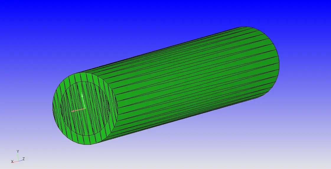
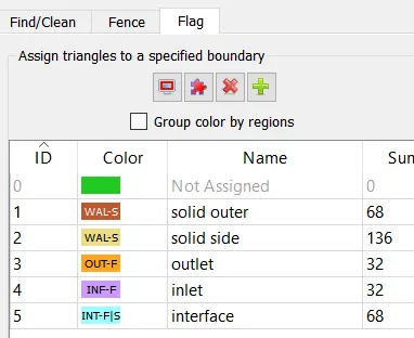
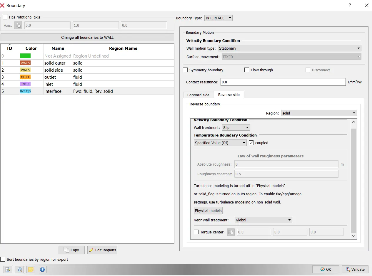
Boundary Flagging:
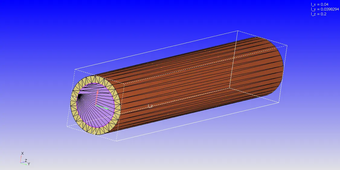
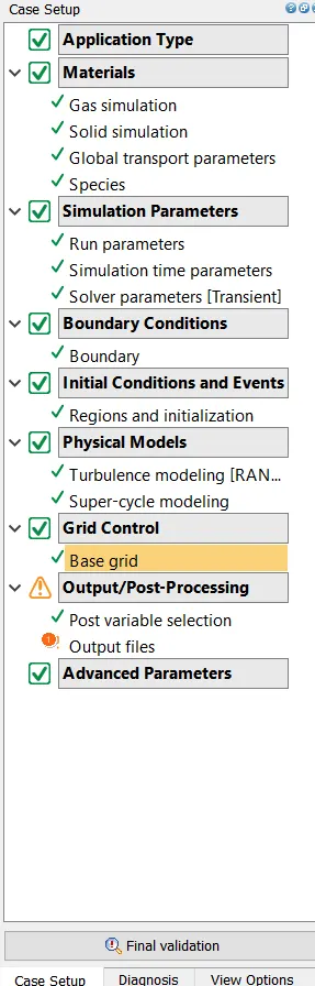
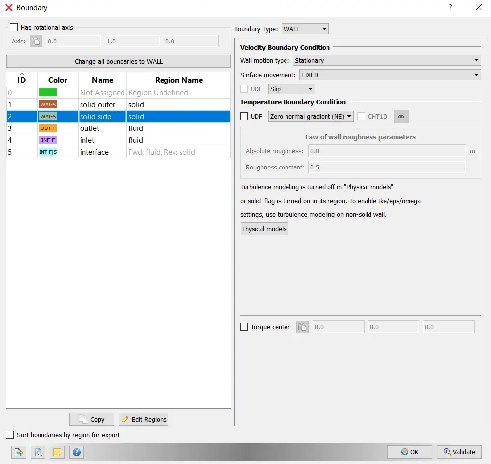
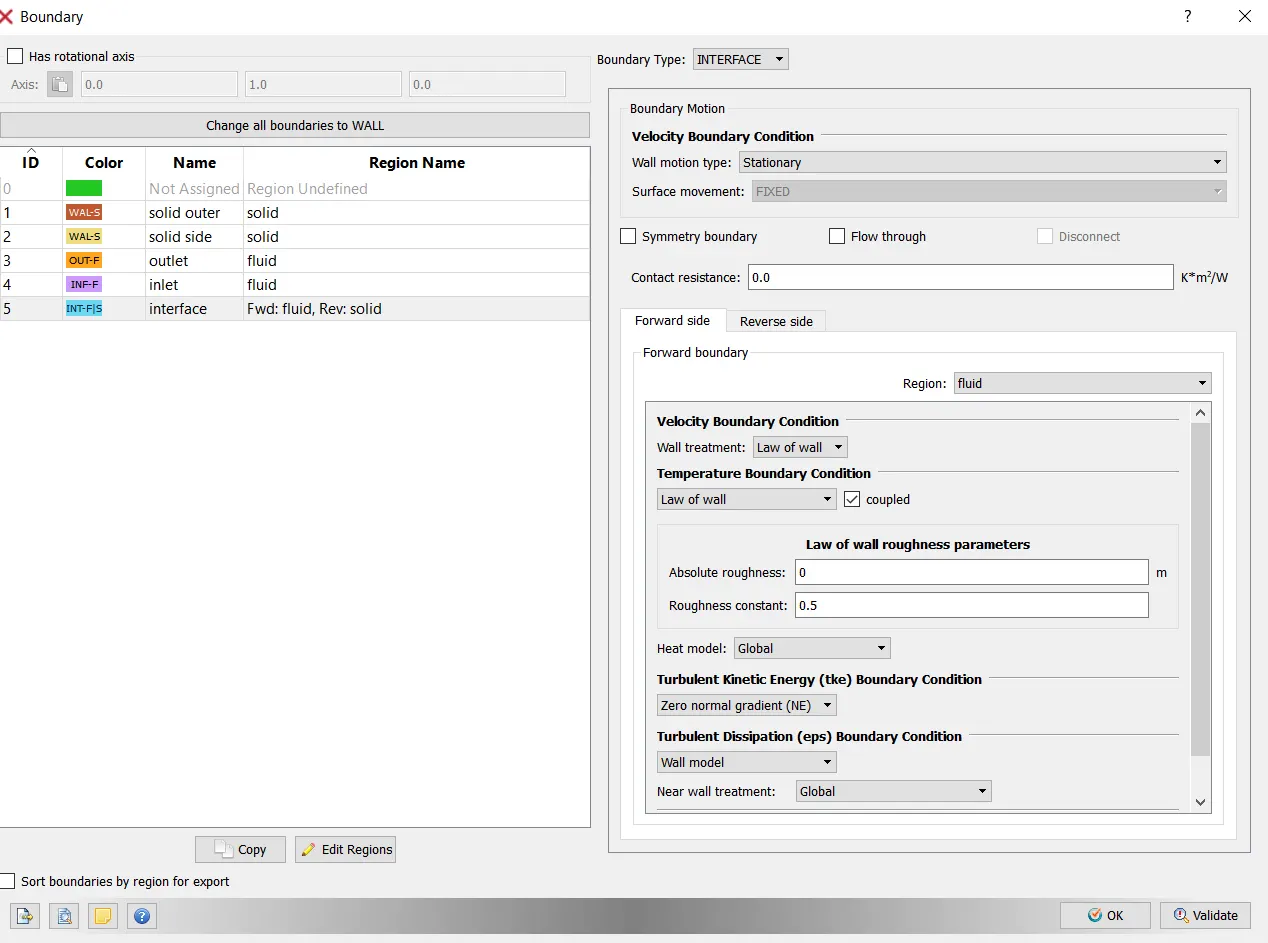
Case setup:
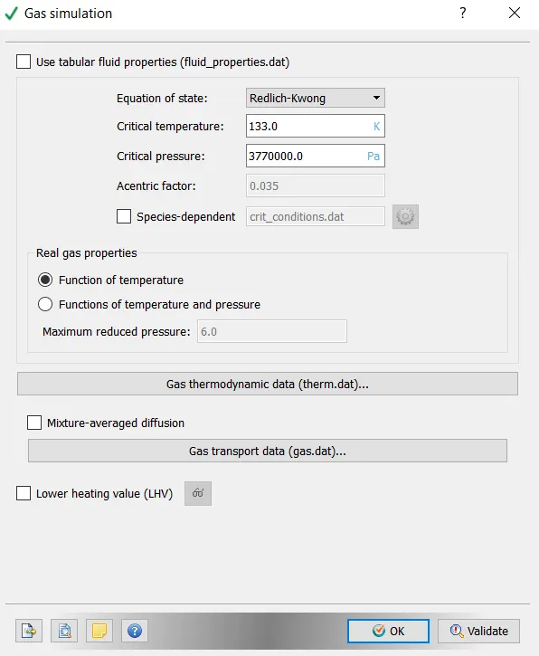
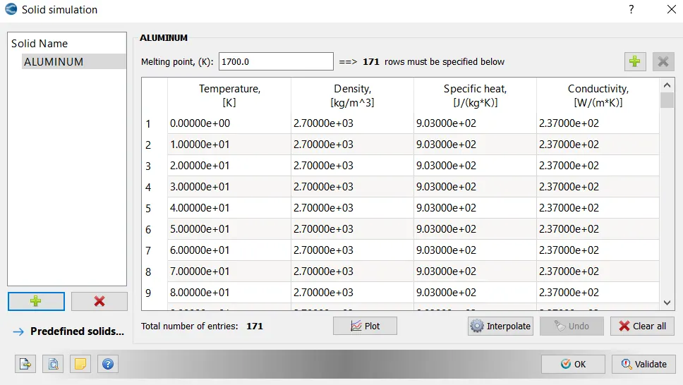
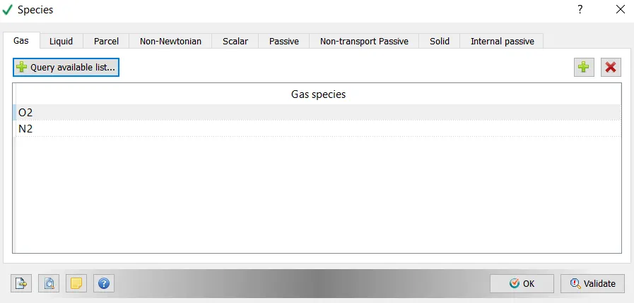
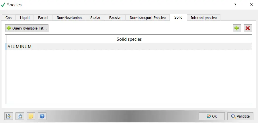
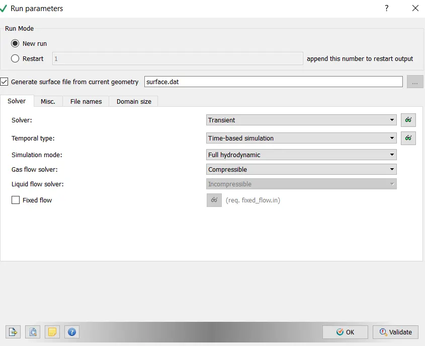
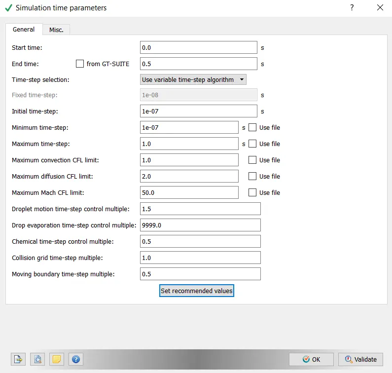
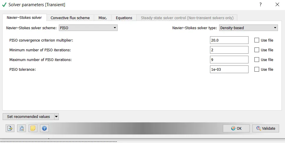
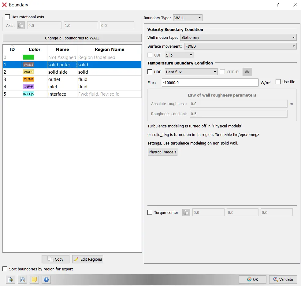
Inlet:
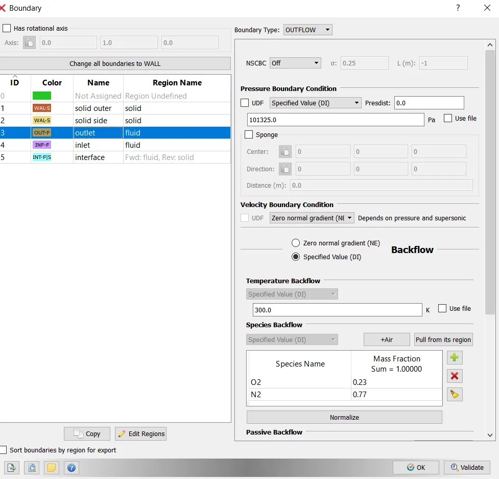
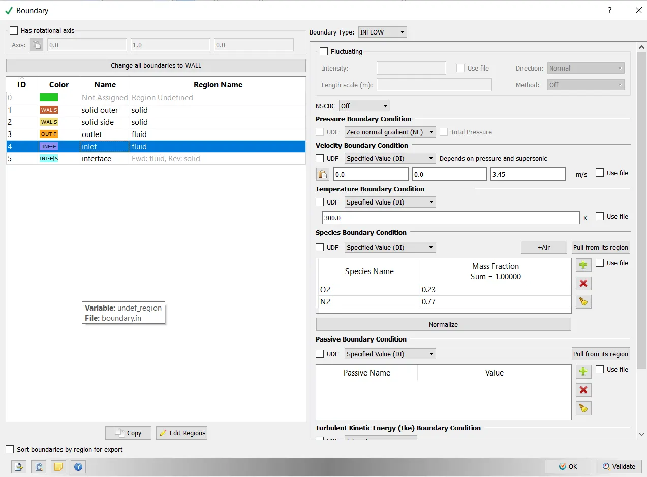
Neumann boundary condition for pressure
Dirchelet boundary condition for velocity. This is calculated usind reynols number=7000
Re = ρ.V.Dμρ.V.Dμ
Re = 7000
Density of air = 1.225 kg/m^3
Viscosity = 1.81e-5 kg.m/s
Hence, Velocity = 3.45m/s
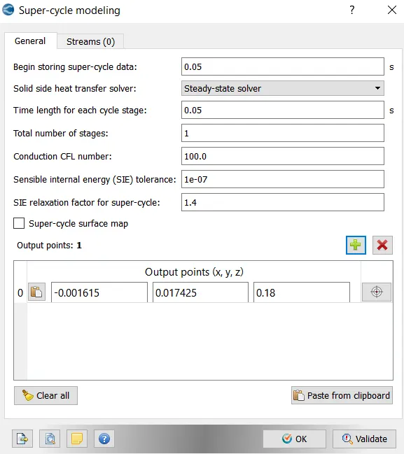
Super-cycle Intervals(sec) Time(sec) Cell-Count
0.01 950.33 13736
0.02 964.23 13736
0.03 957.11 13736
0.05 929.61 6018
The details represent the reduction of simuation time using super-cycling.
Grid-Dependency Test:-
- Grid dependency test carried out in 3 different grid size which are 0.004,0.003,0.002.
Case:1: dx=0.004m dy=0.004m dz=0.004m
Temperature contour
Velocity Contour
Pressure Contour
Animation of Temperature Contour:https://youtu.be/z_FS5sFPZWA
Y+ Contour
Case:2: dx=0.003m dy=0.003m dz=0.003m
Temperature contour
Velocity Contour
Pressure Contour
Animation of Temperature Contour:https://youtu.be/vyJWd84pPSA
Y+ Contour
Case:3: dx=0.002m dy=0.002m dz=0.002m
Temperature Contour
:
Velocity Contour
Pressure Contour
Animation of Temperature Contour:https://youtu.be/c-YDL4f2fCw
Y+ Contour
Plot1:Mean Temperature
Plot 2 :Cell count
Form the grid dependence test it is concluded that the finer mesh gives accurate result. Set super cycle stage interval to 0.01,0.02 and 0.03 For these three values, the total simulation time compare against the baseline configuration increases and iterations also increases with decrease in interval. Y+ value that is obtained for different grid sizes. Y+ value changes from 15 when grid size is 4mm, to around 7 with mesh 2mm. Finally, the optimum super cycle interval for minimum simulation time.