Channel flow simulation using converge CFD software

Aim: To set a channel flow in Converge and post-processing the results, also plot for velocity, cell count, and mass flow rate at inlet and outlet. Provide an animation video for velocity distribution using ParaView.

Objective:

• Running the case for three different base mesh sizes

3 different base mesh sizes are

case1: dx = 2e-4m, dy = 2e-4m, dz = 2e-4m

case2: dx = 1.5e-4m, dy = 1.5e-4m, dz = 1.5e-4m

case3: dx = 1.0e-4m, dy = 1.0e-4m, dz = 1.0e-4m

• Plotting the results mentioned in aim for all the three base cases, Creating a smooth animation for velocity profile.

Introduction:

The channel flow is a general case in which we generally simulate the flow of gases or liquid through a channel/duct and calculate the different properties of flow such as mass flow rate, velocity, pressure, temperature, etc.

For channel flow simulation we can use Converge CFD software to set a case and ParaView for post-processing.

Steps to create a channel flow simulation in Converge and post-processing it:

Step 1: Create a geometry of the channel using create an option in converging with specified dimensions.

Step 2: Conduct a diagnosis to find if there is an error while creating geometry.

Step 3: Setting up a case

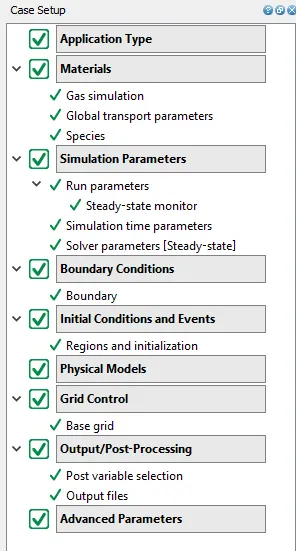
Click on the case set up command the number of parameters that should be defined is being listed in the tree.

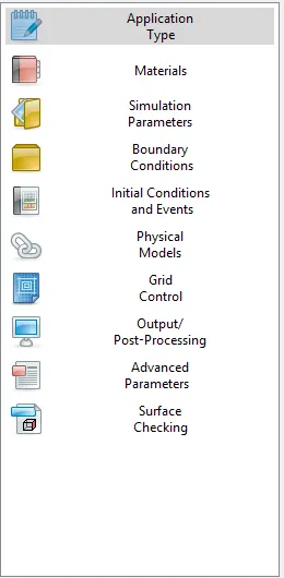
• Select the required dialog box for all the parameters that appear in the case of the setup tree, once selected we can start adding on the values i.e.

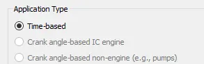
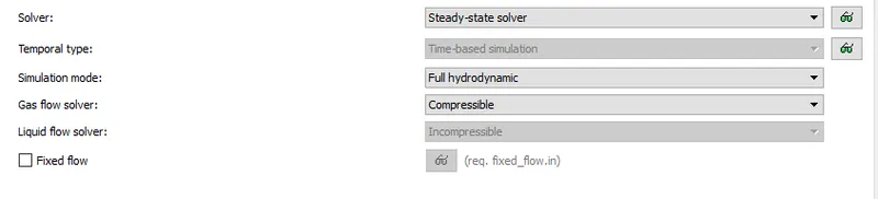
• The first parameter is application type which should be selected as à time base (since we are simulating steady-state simulation)

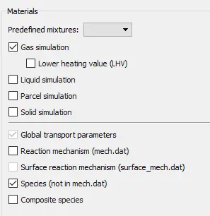
• The next parameters are materials in which we should check the following dialog boxes species, gas simulation, global transport properties, and predefined mixture as air. For gas simulation, and transport properties we should keep the properties as same. In species, we should specify oxygen and nitrogen as major constituents of air.

• Now we add values for simulation parameters in which we should check the following dialog boxes run parameter, simulation time parameters, and solver parameters.

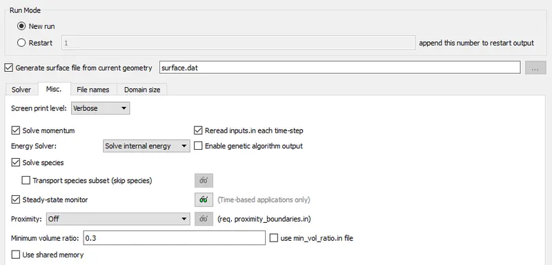
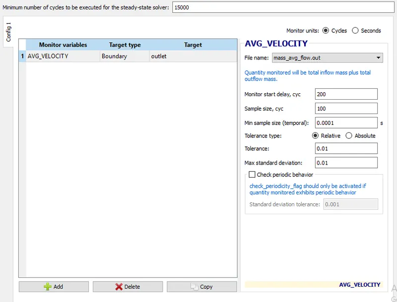
In run parameters, we can also check steady-state monitor box in which we can set parameters i.e. simulation get stopped once convergence is reached hence saving computational time and space and we can monitor any flow properties such as velocity, pressure, density, etc.

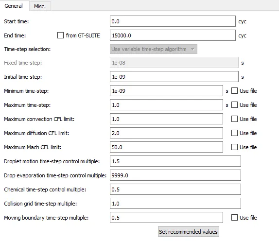
In simulation parameters, we can control start time-end time and time steps also CFL number which actually controls the stability of any solution.

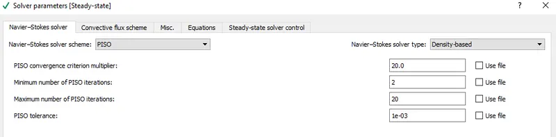
In solver parameters, we will specify the solver scheme and can make choice in b/w density-based or pressure-based solver type.

• It’s Turn to add boundary condition the five boundaries are being named as an inflow (inlet), Outflow (outlet), TWO_D (Front and back), and the wall (top and bottom).
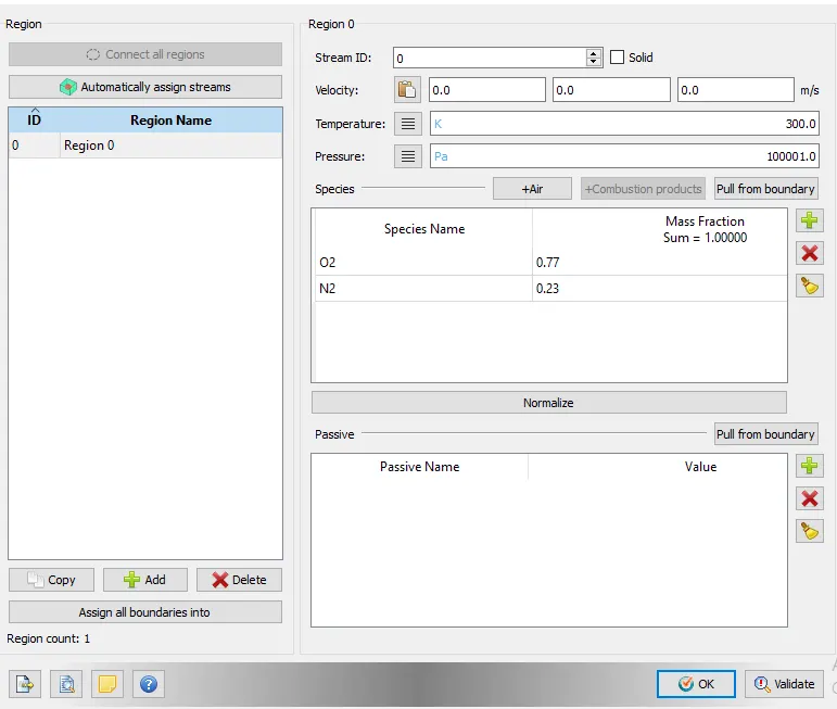
• Now it is a turn to provide a volumetric region on which initial conditions can be applied which can be set inside initial conditions and events in regions and initialization.

• We will not be using a physical model in the case of steady-state simulation.
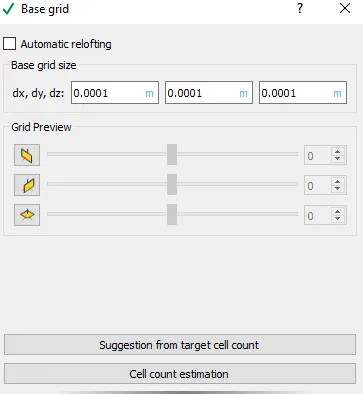
• The next step is to add a grid which can be done in Grid control à base grid.

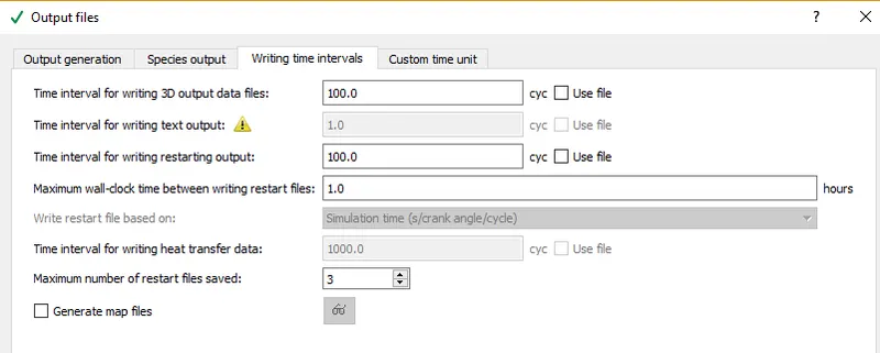
• The final step in case set-up is Output/Post-processing in this section we can define the time interval for writing a 3D – output file such that we can get a maximum number of post-processed files for smooth animation.

Step 4: Saving all the input files in a single folder, and copy the mpiexec.exe file to the folder.

Step 5: Running the simulation using Cygwin.

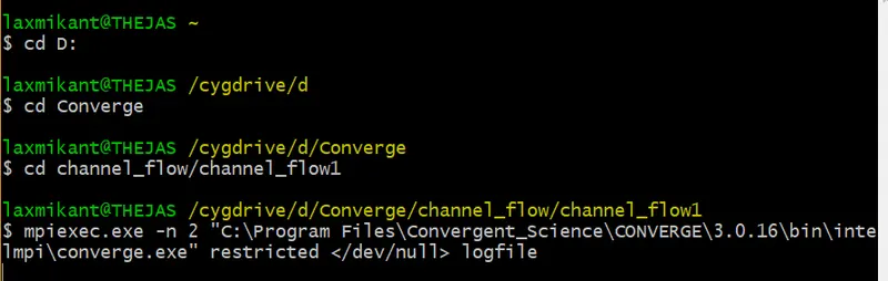
Step 6: Post-processing in Converge in Vtk binary inline format.

Step 7: Visualizing the case in ParaView also saving the animation, contours, and plots.

Mesh for all 3 cases:

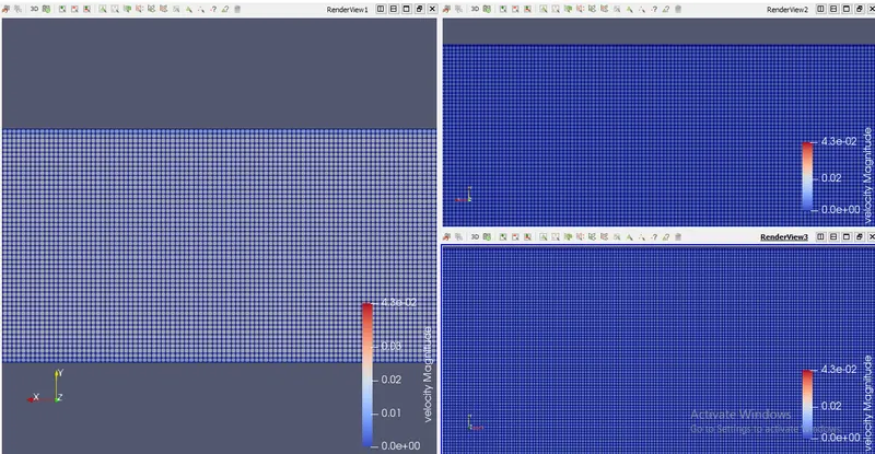
Case1: dx = 2e-4m, dy = 2e-4m, dz = 2e-4m

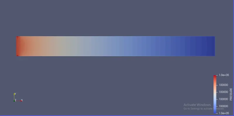
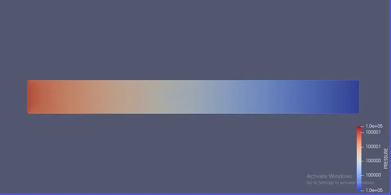
Pressure contour:

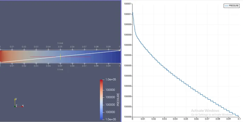
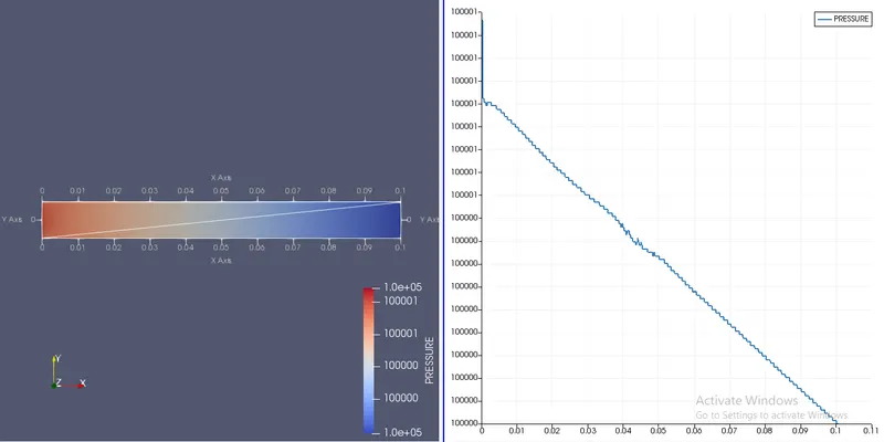
Pressure contour with plot, for variation throughout channel:

Velocity contour:

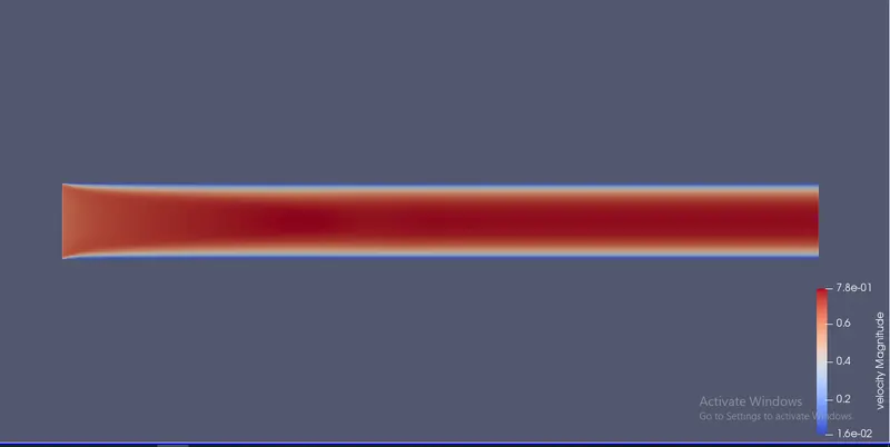
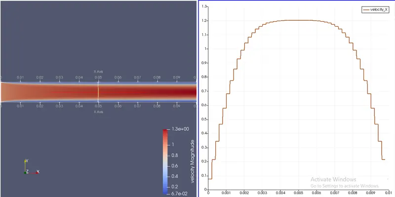
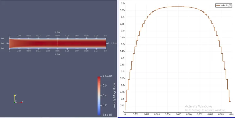
Velocity contour with plot, for variation at 0.05m:

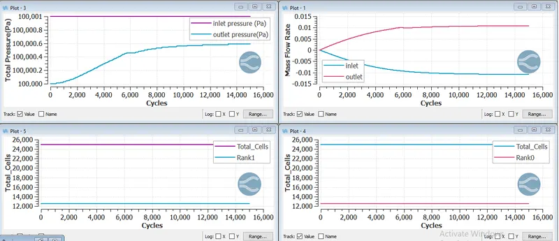
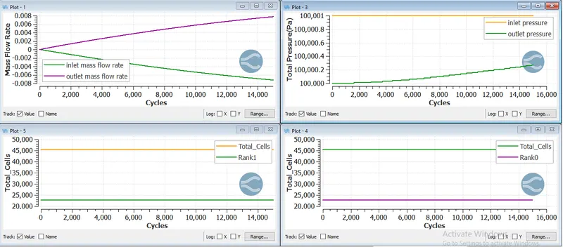
Plots for mass flow rate, Total pressure, and cell count:

Case2: dx = 1.5e-4m, dy = 1.5e-4m, dz = 1.5e-4m

Pressure contour:

Pressure contour with plot for variation throughout channel:

Velocity contour:

Velocity contour with plot, for variation at 0.05m:

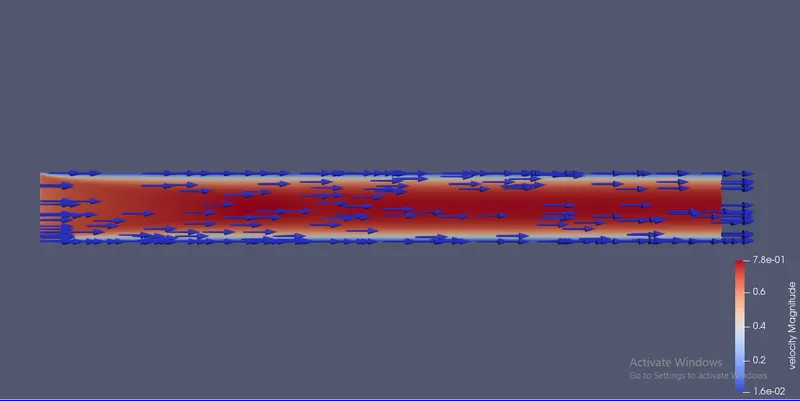
Gylph to estimate the direction of flow with arrows:

Plots for mass flow rate, Total pressure, and cell count:

Case3: dx = 1.0e-4m, dy = 1.0e-4m, dz = 1.0e-4m

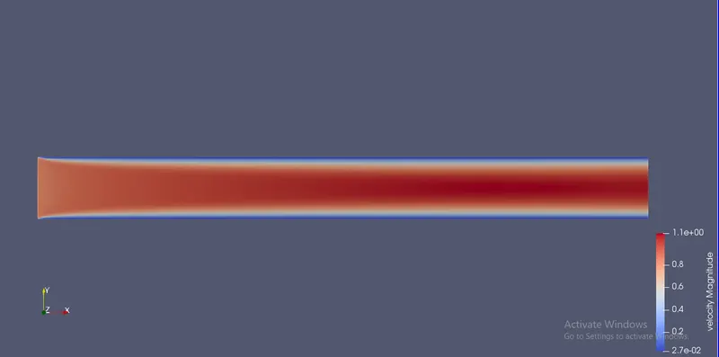
Velocity contour:

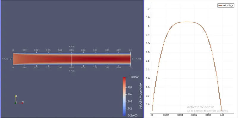
Velocity contour with plot, for variation at 0.05m:

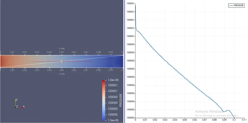
Pressure contour with plot, for variation throughout channel:

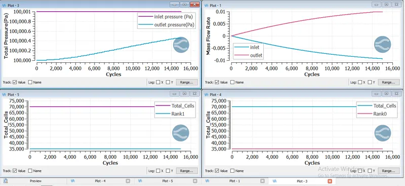
Plots for mass flow rate, Total pressure, and cell count:

Video Link:

https://drive.google.com/file/d/1mqsGGrm6v1_Yhr62G3YhDYHPZO5yJk52/view?usp=sharing

Conclusion:

• The flow takes place only if there is pressure difference, and in direction from higher pressure to lower pressure.
• As the mesh is made finer the cell count increases, and also the accuracy of the solution.
• The flow at the point in the mid-section of channel is parabolic, and fully developed. Also because of no-slip condition applied at wall we see the velocity at vicinity of wall is zero and increases continuously and reaches maxima at center.
• After a particular cycles the flow attends steady state solution.