Challenge: Induction Motor characteristics

Question

1) How induction motor operation is similar to the clutch?

2) Calculate the starting time of a drive with the following parameters:

Answers

#1

Clutch is a mechanical device whose purpose is to temporarily engage or disengage the transmission of rotating power from an input shaft or driving shaft to an output shaft or driven shaft. The clutch provides a transfer of torque between shafts spinning at different speeds, this allows to start moving the vehicle at from a standstill with the engine producing maximum torque at high RPM, this is done by slipping the clutch. When the clutch is disengaged zero power is transmitted and when the clutch is engaged, which means there is full contact between the input and output side, power is directly applied to the output. It is possible to have the clutch engage partially, by allowing the clutch to slip, this results in only a fraction of power to reach the output.

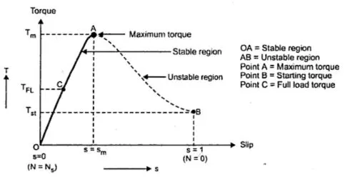
Shown below is the torque slip characteristics of an induction motor,

In a 3 phase induction motor, the stator will generate a rotating magnetic field (RMF) because of the phase shift of 120 degrees within the 3 phase supply input. So the RMF revolves with the stator at its own speed called the synchronous speed. The rotating magnetic field converses with the rotor, so the rotor begins to rotate with a speed which is called actual speed. The disparity between the synchronous speed and actual speed is called slip.

`slip, S = (n_s - n)/n_sxx100`, slip is always expressed in percentage.

`n_s` is the synchronous speed and `n` is the rotational speed.

rotor speed is obtained by reducing slip from stator speed.

Slip varies from 0 at no-load condition to 1 at standstill. From the above curve it can be seen that torque is directly proportional to slip, more the slip more will be the torque produced and vice-versa.

`w_m = w_(ms)(1-S)`

`w_m` is the rotor speed and `w_(ms)` is the stator synchronous speed.

In both the operation of clutch and induction motor, there is slip and loss of power, by this their operations are quite similar.

#2

Given data,

Moment of Inertia of Motor and Load, `J = 10 (kg)/m^2`

Motor Torque, `T_m = 15 + 0.5omega_m`

Load Torque, `T_l = 5 + 0.6omega_m`

In steady state Ideal condition,

`T_m = T_l`

`implies 15+0.5omega_m = 5+0.6omega_m`

`implies 0.1omega_m = 10`

`therefore omega_m = 100` rad/s

Starting time of induction motor is calculated by, `T_m = T_l + J(domega_m)/dt`

from stability equation it can be written as,

`implies 15+0.5omega_m = 5+0.6omega_m + 10xx(domega_m)/dt`

`implies (domega_m)/dt = (10-0.1omega_m)/10 implies 1-0.01omega_m`

`implies dt = (domega_m)/(1-0.01omega_m)`

Time t can be calculated by integrating the above equation.

MatLAB code to calculate the starting time is as follows,

close all
clear all
clc

%Calculating Equilibirum point
w = linspace(0,200,400);    %motor speed
Tm = 15 + 0.5*w;            %motor torque
Tl = 5 + 0.6*w;             %load torque

figure(1)
plot(w,Tm,'linewidth',2)
hold on
plot(w,Tl,'linewidth',2)
grid on
legend('Motor Torque','Load Torque','location','northwest')
title('Speed v/s Torque')
xlabel('Speed - rad/s')
ylabel('Torque - Nm')

%calculating starting time
t_span = [0 1000];
y0 = [0 0];
[t,y] = ode45(@functionmotspeed,t_span,y0);

figure(2)
plot(t,y,'linewidth',2)
grid on
xlabel('Time - s')
ylabel('Speed - rad/s')
title('Motor Speed v/s Time')

Function code is shown below,

function[omega]=functionmotspeed(t,w)
omega = 1-0.01*w;
end

Result

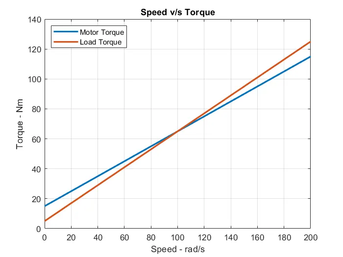
It can be seen from the above plot that the motor torque and load torque converges at `omega_m = 100` rad/s

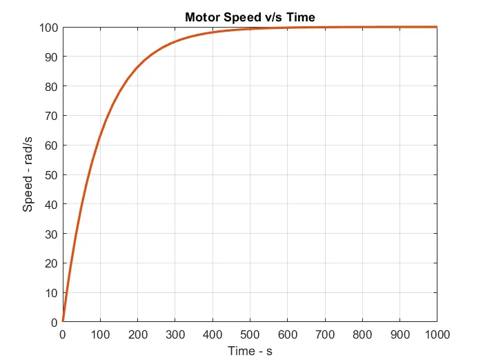
From the above plot it can be noted that the time take to reach 100 rad/s speed is around 600 seconds.

#3

Given data,

`T_m = 1+2omega_m ->(1)`

`T_l = 3sqrt(omega_m) ->(2)`

The condition for stability is given by,

`(dT_l)/(domega_m)-(dT_m)/(domega_m)>0`

MatLAB code to compute the equilibrium point for stability is as follows,

close all
clear all
clc

w = linspace(0,100,5000);   %omega - radians/second
Tm = 1+2*w;                 %motor torque
Tl = 3*sqrt(w);             %load torque

plot(w,Tm,'linewidth',2);
hold on
plot(w,Tl,'linewidth',2);
grid on
ylabel('speed - rad/s')
xlabel('time - sec')
title('Equilibrium point for stability')
legend('Motor Torque','Load Torque','location','northwest')

Result

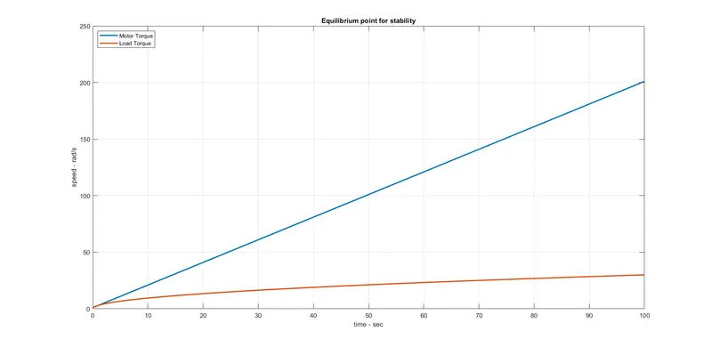
From the plot it can be seen that the two curves intersect each other during the first few seonds, upon zooming the plot the following can be seen.

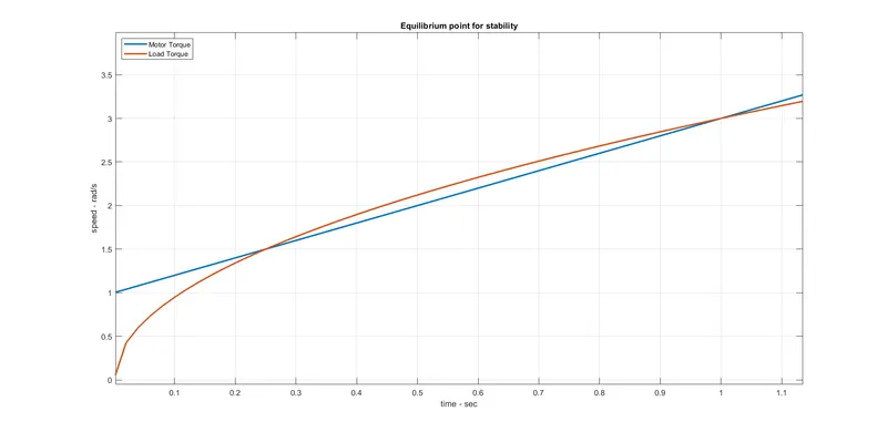
The curves intersect each other at 0.25 second and 1 second mark. so `omega_m` = 0.25 & 1.

Let `omega_m = 0.25`

`(d(3sqrt(omega_m)))/(dt) - (d(2omega_m))/(dt)>0`

upon differentiating we get,

`implies 3/2*omega_m^(-1/2) -2>0`

`implies 3/2*0.25^(-1/2) -2>0`

`implies 1>0` , is true.

Let `omega_m = 1`

differentiating again as done above,

`implies 3/2*omega_m^(-1/2) -2>0`

`implies 3/2*1^(-1/2) -2>0`

`implies -0.5>0`, is not true.

It can be understood that `omega_m = 1` is not an equilibrium point whereas `omega_m = 0.25` is an equilibrium point as it satisfies the condition, `(d(3sqrt(omega_m)))/(dt) - (d(2omega_m))/(dt)>0`.