Breaking Ice with Air cushion Vehicle - Find minimum pressure with Newton-Raphson method
Aim:- Write a python script to solve for the minimum value of pressure of the Air Cushion Vehicle to break the ice bed using the Newton Raphson method.
Objective:-
1. Use the Newton Raphson method to find out the value of pressure for h = 0.6 ft.
2. Find the optimal relaxation factor for this problem with the help of a suitable plot.
3. Tabulate the results of p for h = [0.6,1.2,1.8,2.4,3,3.6,4.2] assuming a suitable relaxation factor. This must be done in python.
Theory:-
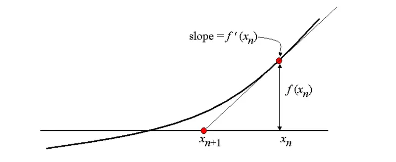
Newton- Raphson Method is a root-finding method which generates approximations of the root of a real function. It uses the idea that a continuous and differentiable function can be approximated by a straight line tangent to it.
Ice sheets can be broken into small slabs with a heavy air-cushion vehicle (ACV) travelling on a float ice sheet at a critical speed. Ice-breaking with ACV is a new ice-breaking method in the In-land River which has important applications in the prevention of ice jam floods.
How does it work?
1. To start with, we assume an initial guess which is closer to the true root of the given function.
2. Find the value of the function at this initial guess.
3. Find the slope of the tangent at this point using calculus to find the x-intercept of this tangent.
The obtained x-intercept is a better approximation for the true roots than the initial guess value. And then this process is repeated until we start getting closer values up to a certain tolerance after the decimal point.
Let f(x) = 0 is a function,
Let initial value of root be `x_0`
Then the f(`x_0`) is the value of the function at `x_0`
Now, the approximate value `x_"new"` is given by
`x_"new"=x_0 - f(x_0)/(f'(x_0)`
Now, the new value of x is taken as the initial value of x and the above process is repeated to get the next approximation. This process is repeated until we get the most approximate value of the true roots.
1. Use the newton raphson method to find out the value of pressure for h = 0.6 ft.
The program for finding out the value of pressure for h=0.6 ft is given below,
import math
import matplotlib.pyplot as plt
import numpy as np

##Inputs
beta=0.5 ## related to width of ice wedge
r= 40 ##size of air cushion in feet
sigma = 21600 ##tensile strength of the ice in pounds per square feet
h= 0.6 ##thickness of the ice field in feet

##Defining governing equation

def f(p,beta,h,r,sigma):
	term1 =pow(p,3)*(1-pow(beta,2))
	term2 =pow(p,2)*((0.4*h*pow(beta,2))-(sigma*pow(h,2))/pow(r,2))
	term3= p*((pow(sigma,2)*pow(h,4))/(3*pow(r,4)))
	term4=(sigma*pow(h,2))/(3*pow(r,2))
	T1=term1+term2+term3-pow(term4,3)
	return T1

##Defining the derivative of governing equation

def fprime(p,beta,h,r,sigma):
	term5 =3*pow(p,2)*(1-pow(beta,2))
	term6 =2*p*((0.4*h*pow(beta,2))-(sigma*pow(h,2))/pow(r,2))
	term7= ((pow(sigma,2)*pow(h,4))/(3*pow(r,4)))
	T2=term5+term6+term7
	return T2

##Performing the Newton Raphson Method

p_guess=100
alpha = 0.8 ##relaxation factor taken below 1 in this case
tol=1e-5
iter =1
while(abs(f(p_guess,beta,h,r,sigma))>tol):
	p_guess= p_guess - alpha*(f(p_guess,beta,h,r,sigma)/fprime(p_guess,beta,h,r,sigma)) ##pressure in pounds per square feet
	iter=iter+1

print(iter)
p_final = p_guess/144 ##Pressure in pounds per square inch
print(p_final)
Result:-
After running the above code, the following results were obtained.

2. Find the optimal relaxation factor for this problem with the help of a suitable plot.
The program for finding the optimal value of the relaxation factor is as per below,
import math
import matplotlib.pyplot as plt
import numpy as np

##Inputs
beta=0.5 ## related to width of ice wedge
r= 40 ##size of air cushion in feet
sigma = 21600 ##tensile strength of the ice in pounds per square feet
h=0.6 ##thickness of the ice field in feet
###h = [0.6,1.2,1.8,2.4,3,3.6,4.2] ##thickness of the ice field in feet

##Defining governing equation

def f(p,beta,h,r,sigma):
	term1 =pow(p,3)*(1-pow(beta,2))
	term2 =pow(p,2)*((0.4*h*pow(beta,2))-(sigma*pow(h,2))/pow(r,2))
	term3= p*((pow(sigma,2)*pow(h,4))/(3*pow(r,4)))
	term4=(sigma*pow(h,2))/(3*pow(r,2))
	T1=term1+term2+term3-pow(term4,3)
	return T1

##Defining the derivative of governing equation

def fprime(p,beta,h,r,sigma):
	term5 =3*pow(p,2)*(1-pow(beta,2))
	term6 =2*p*((0.4*h*pow(beta,2))-(sigma*pow(h,2))/pow(r,2))
	term7= ((pow(sigma,2)*pow(h,4))/(3*pow(r,4)))
	T2=term5+term6+term7
	return T2

##Performing the Newton Raphson Method


## Taking underrelaxing and overrelaxing values for alpha array
alpha_initial=0.1
alpha= []
for a in range(0,30):
	alpha_initial = alpha_initial + 0.06
	alpha.append(alpha_initial)
iterations=[]

for i in alpha:
	p_guess=100
	tol=1e-5
	counter =1
	while(abs(f(p_guess,beta,h,r,sigma))>tol):
		p_guess= p_guess - i*(f(p_guess,beta,h,r,sigma)/fprime(p_guess,beta,h,r,sigma)) ##pressure in pounds per square feet
		counter=counter + 1
		p_final=p_guess/144
	iterations.append(counter)

for k in range(len(iterations)):
	if iterations[k]==min(iterations):
		print("The optimum value of Relaxation Factor: ", str(alpha[k]))

plt.figure(1)
plt.plot(alpha,iterations,marker=".",color='red',markersize=5)
plt.xlabel("Relaxation Factor (Alpha)")
plt.ylabel("No. of Iterations")
plt.title("Iterations Vs Relaxation Factor")
plt.show()
Result:-

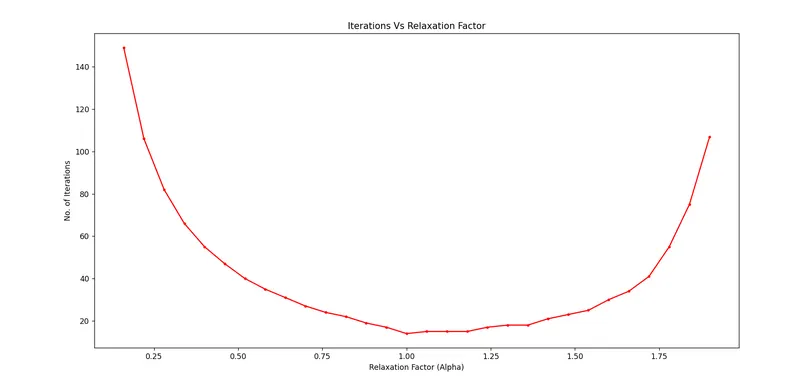
It can be concluded that No. of iterations decreases rapidly with an increase in the Relaxation factor and again increases later on. Closely looking into the graph, one may comprehend that No. of iterations varies minimally near the relaxation factor of 1. And hence the most optimal value comes out to be very close to 1.
3. Tabulate the results of p for h = [0.6,1.2,1.8,2.4,3,3.6,4.2] assuming a suitable relaxation factor. This must be done in python.
The program for the above is as shown below
import math
import matplotlib.pyplot as plt
import numpy as np

##Inputs
beta=0.5 ## related to width of ice wedge
r= 40 ##size of air cushion in feet
sigma = 21600 ##tensile strength of the ice in pounds per square feet
h = [0.6,1.2,1.8,2.4,3,3.6,4.2] ##thickness of the ice field in feet

##Defining governing equation

def f(p,beta,h,r,sigma):
	term1 =pow(p,3)*(1-pow(beta,2))
	term2 =pow(p,2)*((0.4*h*pow(beta,2))-(sigma*pow(h,2))/pow(r,2))
	term3= p*((pow(sigma,2)*pow(h,4))/(3*pow(r,4)))
	term4=(sigma*pow(h,2))/(3*pow(r,2))
	T1=term1+term2+term3-pow(term4,3)
	return T1

##Defining the derivative of governing equation

def fprime(p,beta,h,r,sigma):
	term5 =3*pow(p,2)*(1-pow(beta,2))
	term6 =2*p*((0.4*h*pow(beta,2))-(sigma*pow(h,2))/pow(r,2))
	term7= ((pow(sigma,2)*pow(h,4))/(3*pow(r,4)))
	T2=term5+term6+term7
	return T2

##Performing the Newton Raphson Method
pressure=[]
alpha=0.85
iterations=[]

for i in h:
	p_guess=100
	tol=1e-5
	counter =1
	while(abs(f(p_guess,beta,i,r,sigma))>tol):
		p_guess= p_guess - alpha*(f(p_guess,beta,i,r,sigma)/fprime(p_guess,beta,i,r,sigma)) ##pressure in pounds per square feet
		counter=counter + 1
		p_final=p_guess/144
	pressure.append(p_final)

	iterations.append(counter)

print("Thickness of Ice field (in feet)",h)
print("Cushion Pressure (PSI) ",pressure)

plt.figure(1)
plt.plot(h,pressure,marker=".",color='red',markersize=5)
plt.xlabel("Thickness of Ice Field(feet)")
plt.ylabel("Pressure (PSI)")
plt.title("Pressure Vs Thickness of Ice Field")
plt.show()
Result:-
The values of Cushion pressure for different values of thickness of ice field are plotted below.

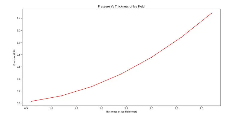
From the above, we can see that the pressure increases with an increase in the thickness of the ice field.
Conclusion:-
All objectives are worked upon and all results are discussed as aforementioned.
References:-