Basics of ML & AL Week 2 Challenge

Solution 1:

Random Variable number of toys X	Probability of selling toys P(X)	First Business Moment `Sigma(x)*P(x)`	Second Business Moment `sigma^2=Sigma (x - mu)^2 *P(x)`	Third Business Moment `S_k`=`Sigma ((x - mu )/sigma)^3 *P(x)`	Fourth Business Moment `K_t = Sigma ((x - mu)/sigma)^4*P(x) -3`
0	0.35	0	0.686	-0.384791453	-2.6
1	0.25	0.25	0.04	-0.00641052	-3
2	0.15	0.3	0.054	0.012981303	-2.99
3	0.15	0.45	0.384	0.246163962	-2.71
4	0.1	0.4	0.676	0.704195604	-1.65
		`mu`=1.4	`sigma^2`=1.84	`S_k =`0.572138895	`K_t`-13
		Standard Deviation (`sigma`)	1.356465997

Solution 2

Expected Value: When we want to calculate the mean of a probability distribution this gives the average value we expect to occur before collecting the data.

Mean: It is the average value of the collected data sample.

solution 3

Having skewness in the curve considered to be bad in the analysis?

First, understand what we mean by skewed data, we call data to be skewed when the normal distribution of the data is shifted to the left or right side as shown in below figure.

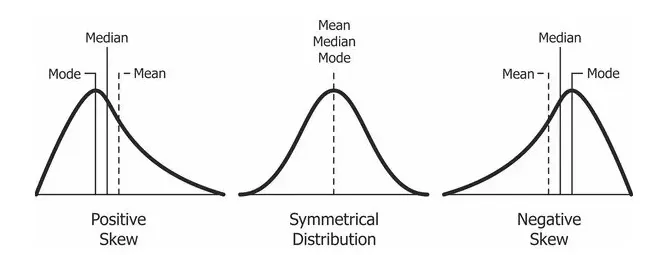
Positive skewed: Data is said to be positively skewed if the tail on the right side is more extended and flatter than the left side.

Negative skewed: Data is said to be negatively skewed if the tail on the left side is more extended and flatter than the right side.

In real-world applications, the data is always skewed but too much-skewed data tells us that it will adversely affect the model performance, especially regression-based models. While there are statistical models that are robust enough to handle outliers like tree-based models, you’ll be limited in what other models you can try. So what do you do? In order to fit the models we need to transform the data so that it will become the gaussian ( normal ) distribution.

Solution 4

Evaluate the probabilities for continuous normal distribution with given mean = 680 and standard deviation = 31

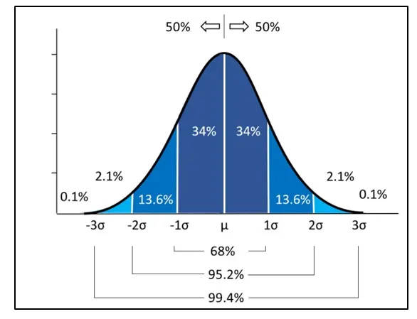
a)P(X<711)

Here the Z values is

`Z = (x - mu) /sigma`

= (711 - 681)/31

= 1

so according to the graph P(X < 711 ) = 50 + 68/2 = 84 %

b)P(X>740)

Z = 1.93

so probability is P(X>740) = 2.2 %

c)P(600<x<720)

Z1 = ( 600 - 680 ) /31

= -2.58

Z2 = ( 720 -680 )/31

= 1.29

P(600<x<720) = 89.65 %

d)P(X=720)

Z = 720-680/31

= 1.29

P(X=720) =

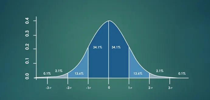
The curve shown in above figure is known as normal distribution or the bell curve in which shows that

1) 68% of all values are within one standard deviation of mean values

2) 95 % of all values are within two standard deviation of mean values

3) 99% of all values are within three standard deviation of mean values

4) this curve shows the probability density of data set of occurring certain value, total area under the curve will be equal to 1.

• The normal distribution is the proper term for a probability bell curve.
• In a normal distribution, the mean is zero and the standard deviation is 1. It has zero skew and kurtosis of 3.
• Normal distributions are symmetrical, but not all symmetrical distributions are normal.
• Many naturally-occurring phenomena tend to approximate the normal distribution.