Basic function modeling and analysis of 'Suspension System Comparison' model using SIMULINK

Objectives:

1. Plotting a function using Simulink blocks
2. Analysis of a simulink model

#Objective A:

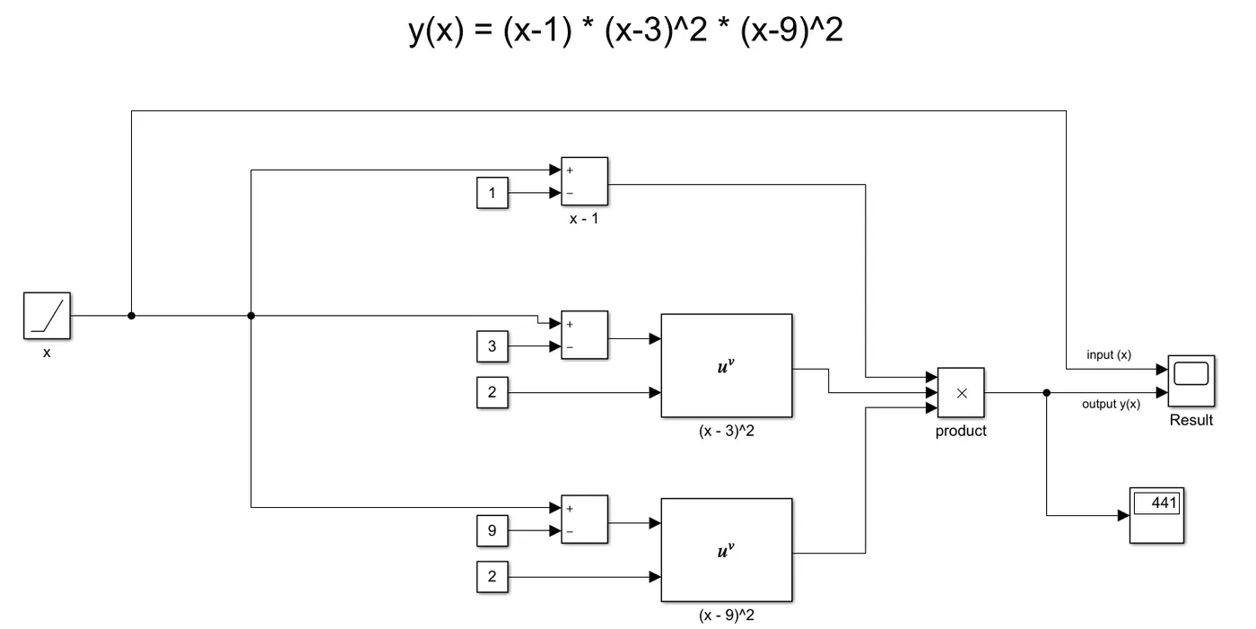
The function to be plotted is:

`y(x) = (x-1)(x-3)^2(x-9)^2`

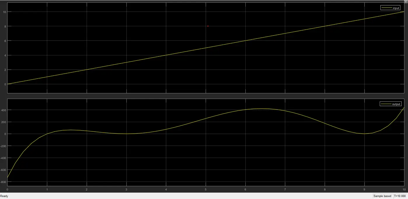
Graphical result:

#Objective B: Analysis of 'Suspension System Comparison'

Theory and Background:

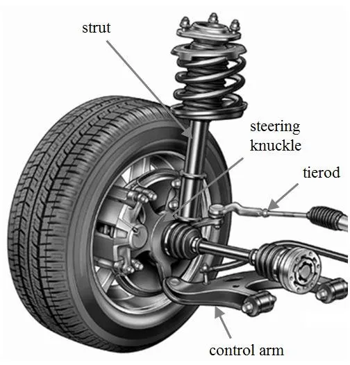
Suspension system is the combined system of tires, springs, shock absorbers, and linkages that connects the body to the wheels and allows the aggregated motion of the vehicle. The main requirements of the suspension system include, but are not limited to:

• Maximizing friction between the tires and the road surface during acceleration, cruising, and braking
• Provide steering stability with good handling
• Comfort of the passengers

The model below will be the discussion centrepoint

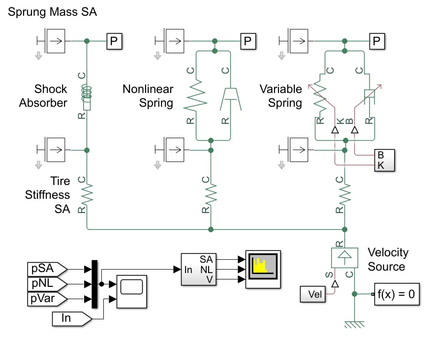
The different types of suspensions, as also seen in the model above include, but are not limited to:

• Shock absorbers

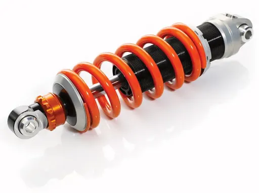
A mechanical device designed to absorb and reduce vibrations in the spring by converting the kinetic energy generated into heat, dissipated through hydraulic fluid. Most shock absorbers are a form of dashpot; a damper that resists motion due to friction

• Linear and Non-Linear springs

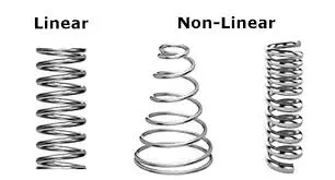
Non-linear springs exert an inconsistent amount of force when under a load, unlike linear springs, which follow Hooke's law.

• Variable springs

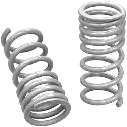
As is evident in the figure, variable springs are tightly sprung in some areas and loosely strung in others, giving a variation in spring stiffness.

With reference to the simulation model above, the objective of the simulation is to compare the results of three different types of suspension systems, based on springs and shock absorber, that are driven by a common velocity source. The three systems can therefore be compared.

Similarities:

• Common oscillating velocity source
• Same tire stiffness i.e. 2e5 N/m
• Values of sprung mass (350kg) and unsprung mass (50kg) are identical

Differences:

• Three different suspensions are used for comparison i.e. translational shock absorber, non-linear spring, and variable spring. This certainly will generate a different amount of stress and displacement in the body in all three studies.

Output of the simulation: Sprung mass position and input velocity

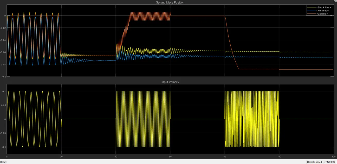
The plots above show the position of the sprung masses in the individual setups that were subjected to the same test.

Observations:

• For the initial 20 seconds, the sprung mass has similar variation in position for all three studies.
• The pulse is absent from 20-40 seconds, and therefore the dispplacement is negligible
• During 40-60 seconds, the second pulse, variable spring undergoes the highest amount of variation in displacement, while the other two are fairly constant.
• The pulse is absent from 60-80 seconds
• For 80-120 seconds, the variable spring experienced the least amount of distortion
• Overall, the shock absorber and the non-linear spring display a pretty stable nature.

Power spectral density vs Frequency:

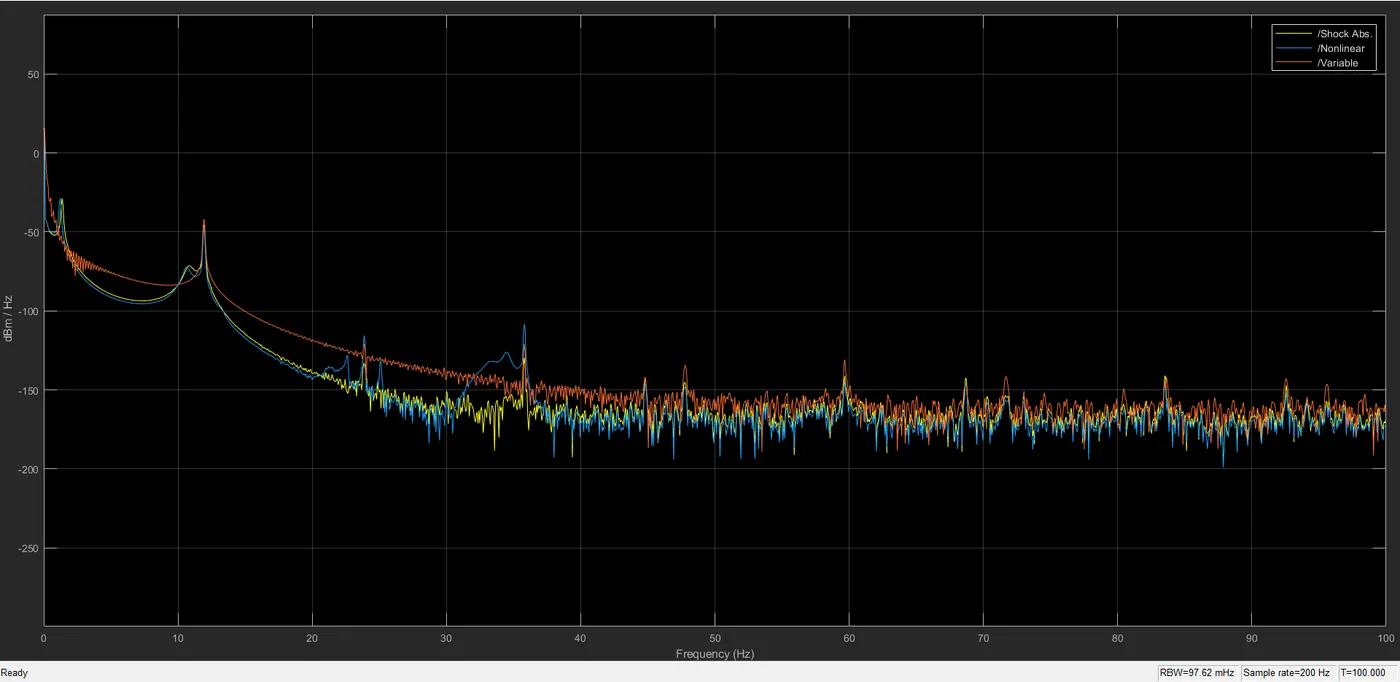
Using a spectrum analyser, the above plot demonstrates that as frequency of the oscillating velocity increases, the power spectral density decreases i.e. noise levels per frequency.

How is an oscillating velocity source created?

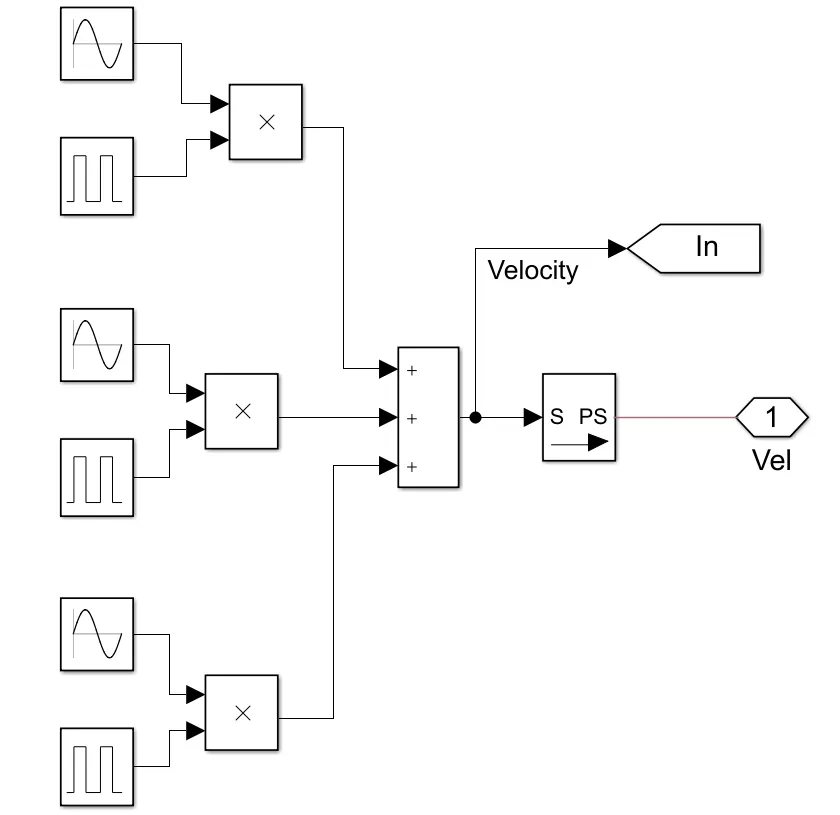
It is created using sin wave and pulse generator blocks. For testing purposes, the suspension systems were to be subjected to oscillating velocities of different frequencies, so two additional sets of sin waves and pulse blocks were added. The frequencies of the sin wave blocks were 3 rad/sec, 15 rad/sec, and 75 rad/sec, respectively. The output is merged together and passed through a Simulink-PS converter to turn the input signal into a physical signal.