Side Pole Impact Analysis of NEON Doge Model in FMVSS Regulation

OBJECTIVE

Performing Side pole crash analysis of a car

PROCEDURE

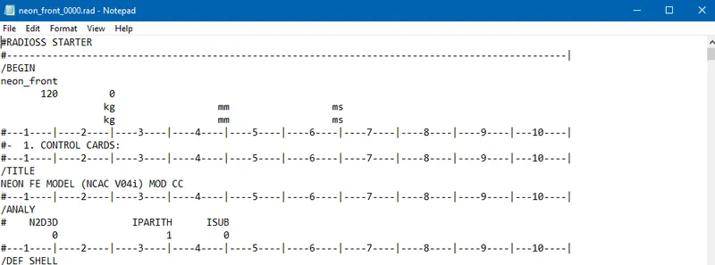
1. The unit system in place is [Kg mm ms]. Open the 0000.rad file in notepad and one can observe the unit system in the starter file.

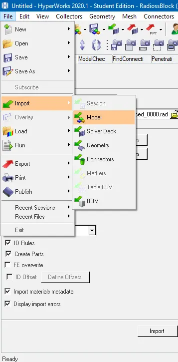
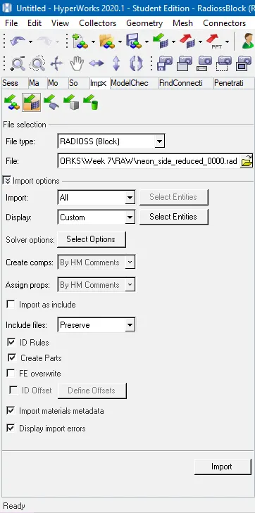
2. Open the file in the HyperWorks, select the Radioss solver and import the neon_side_reduced_0000.rad file. K Run the model checker to see for the errors and warnings throughout the file. We can solve them one by one.

3. We will delete the existing contact interfaces and then create a new Type 7 contact interface with recommended parameters as shown below.

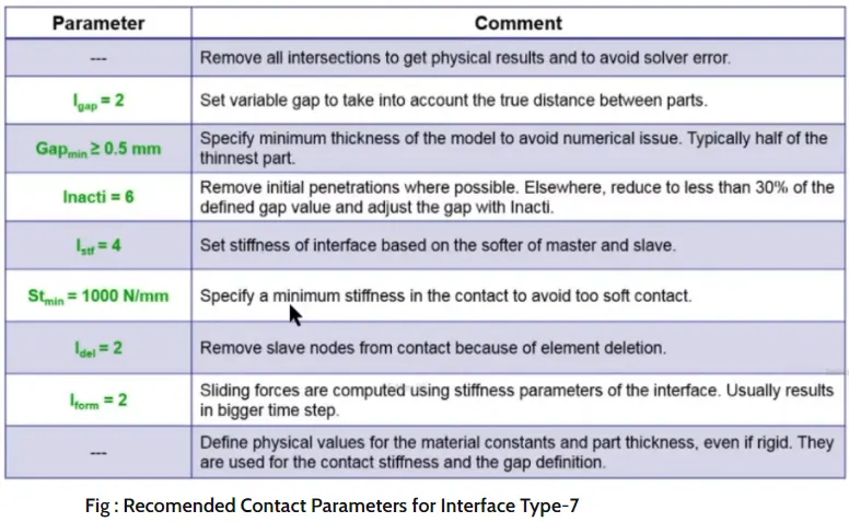
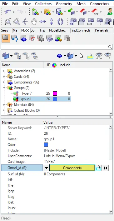
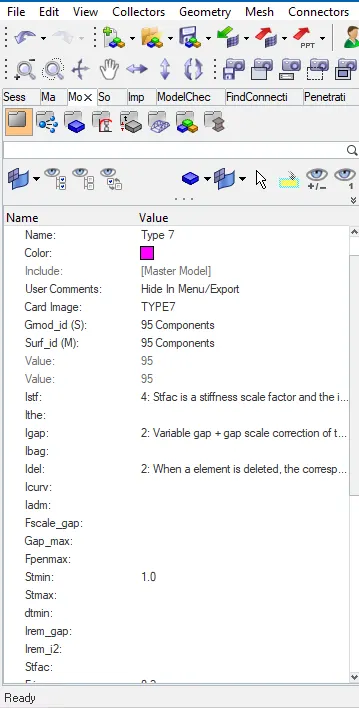
4. Under the Model tab, right-click to create a new group. Select Card Image as TYPE 7 and then for master and slave entity IDs, choose the option as component and select all available components. Populate the recommended parameters.

5. Make sure of no penetrations and intersections. Penetration is defined as the overlap of the material thickness of the shell elements, while Intersection is defined as elements that actually pass completely through one another. All models and especially impact models should be checked for penetrations and intersections and de-penetrated to ensure the integrity of the model. Penetrations adversely affect results and should be removed.

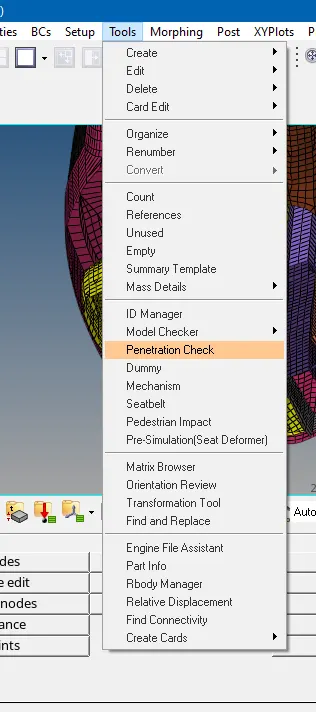
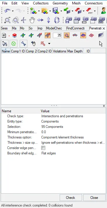
6. Right-click on the tools tab and select the penetration test. Select the entity type as components and do the necessary selections. Go for the check. No collision found and hence no penetration and interaction found in the model.

7. Now we will look at the material property and make some necessary changes if required as per recommendation. The material cards are mostly LAW 2(M2_PLAS_JOHNS_ZERIL) or Johnson Cook which is an elastoplastic material. This workload involves nonlinear analysis which requires the value of true stress and true strain. In this law, the material behaves as linear elastic when the equivalent stress is lower than the yield stress. For higher stress values the material behavior is plastic.

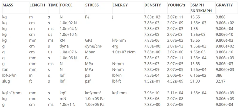
8. We will use consistent units to check out the material property. The unit system in place is [KN mm ms Kg] and the value of density, youngs modulus are in accordance with that of steel.

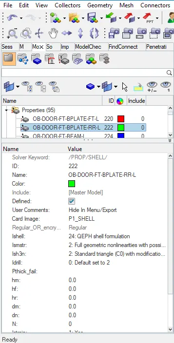
9. We will take a look at the shell element formulation property to ensure it is in line with the recommendation. Make some necessary changes as required.

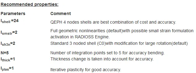
10. With a one-point integration formulation, if the non-constant part follows exactly the state of the constant part for the case of elastoplastic calculation, the plasticity will be under-estimated due to the fact that the constant equivalent stress is often the smallest one in the element and element will be stiffer. Therefore, QEPH, defining a yield criterion for the non-constant part seems to be a good idea to overcome this drawback. QEPH shells are more accurate for elastic or elasto-plastic loads, whatever the loading type - quasi-static or dynamic. QEPH shells will give better results if the mesh is fine enough. It is not recommended for the coarse mesh.

11. In the case of elastic behavior, one gets the exact solution from three integration points – that is to say that the bending moments are exactly integrated through the thickness of the shell – and it is not necessary to use more integration points. In the case of plastic behavior, the bending moments are not integrated exactly. Using more integration points, the solution becomes more accurate; so it is recommended to use five integration points and N=0 means the global integration method is applied(Each element is integrated based upon its property). The default value is 0 which means the global integration model which only compatible with Material Laws 1, 2, 22, 36, 43, and 60. Failure models are not available with global integration for shells.

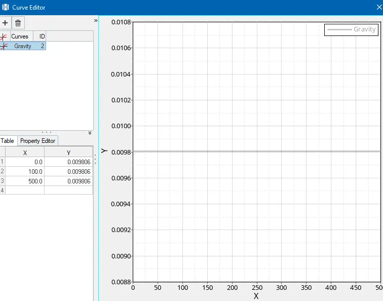
12. We will create a curve function for our gravity fct_ID. In the model tab, right-click to create a curve and define the time function like 0 to 500 ms with the gravity of 9.806e-03 keeping it with consistent units.

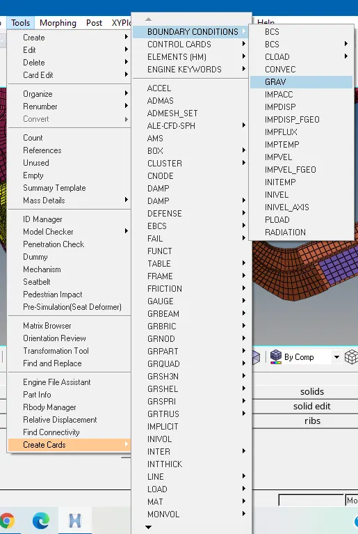
13. We need to define the gravity for the model. Under the Tools tab, select create card option and choose the Boundary conditions.

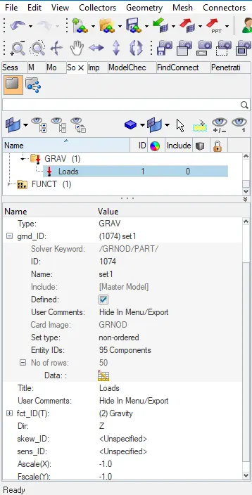
14. For Grnod_ID right-click to create a new one. Keep the entity ID as components and select every component. Select the Dir as Z-axis and change the Ascale and Yscale as -1.0. Keep the Skew_ID as none to use the global co-ordinate system.

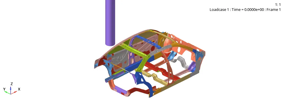
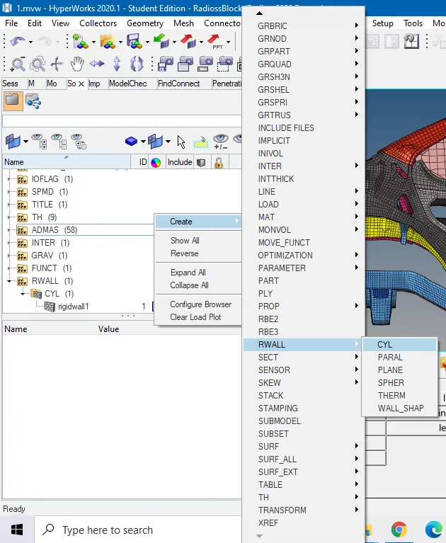
15. We will now create the rigid wall in form of a Cylinder upon which the side impact will take place. Right-click under the solver tab and select the RWALL with cylinder option. Select the Slide as 2 to have a sliding with friction option.

16. Give proper coordinates to keep the pole upright and some distance away from the door to simulate the impact. It will feature a recommended friction value of 0.1, Dsearch as 1000, and diameter as 254 mm which is the standard value.

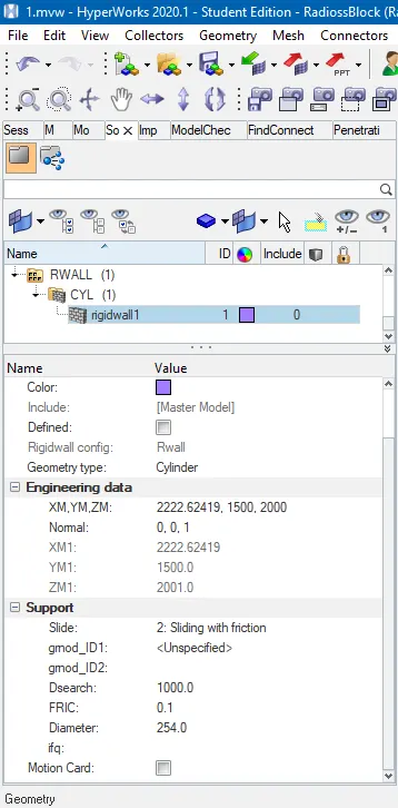
17. A rigid wall is a nodal constraint applied to a set of slave nodes in order to avoid the node penetration to the wall. If contact is detected, then the slave node acceleration and velocity are modified.

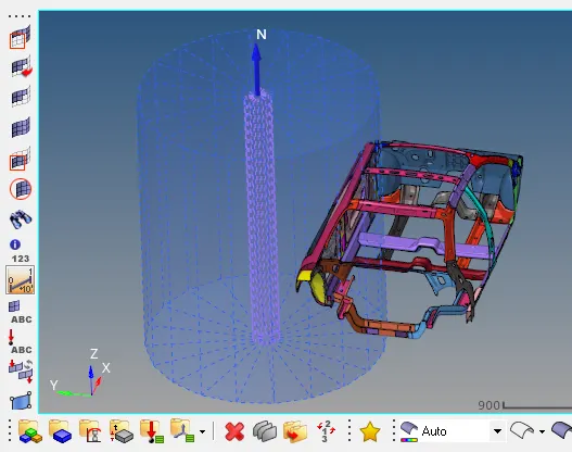
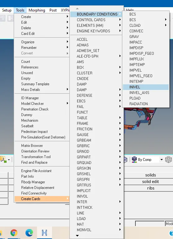
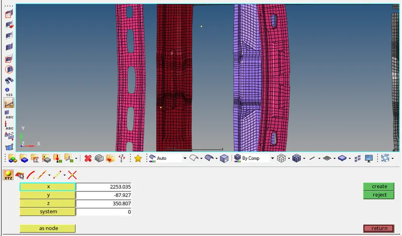
18. Now we will apply the necessary initial velocity to the model so that the BIW can make the contact with the pole. Under the Tools tab, go to the Boundary conditions option, and click Invel.

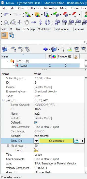
19. Click on create a new grnod_ID and keep the entity ID as components. Select all components and keep the type as TRA(Translational Material Velocity) and Y-axis Velocity as 15.65. Velocity value is aligned with the consistent units [Kg mm ms] and we are keeping the initial velocity as 35 MPH.

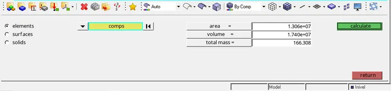
20. Now we will check the mass of the body. Click on the mass calc option under the tool tab and select all the components for mass calculation. We find the mass to be around 166.308kgs. We will need to increase it to 700 Kg and bring the CG position right below the front seating while maintaining the same CG coordinates value on the Y and Z axis.

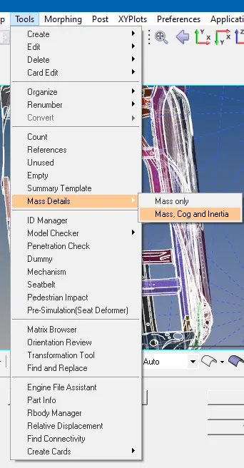
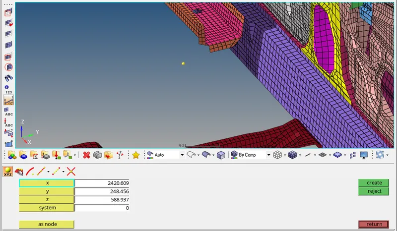
21. Now we will check for the position of CG for the car. Select on Mass details option under the Tools tab to get the position of the COG. Plot the coordinates with a node to get a visual confirmation for the position. Select the nodes option present under the geometry tab to get the same.

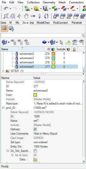
22. Click on Admas present under create cards option of tools tab and select the option to create a new mass. Pick Type 1 as it leads to mass distribution to each node of the node group. For Grnod right click and create new select the required nodes. Add the necessary mass as required.

23. Keep on adding the admas until you get the required mass of 700kgs and then inspect the coordinates of CG. Plot the coordinates with a node to get a visual confirmation for the position. We need the CG position in such a way that it mimics the fully laden vehicle to make sure practical vehicle dynamics characteristic.

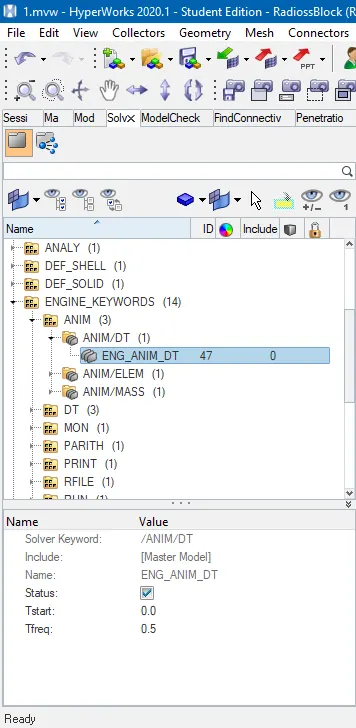
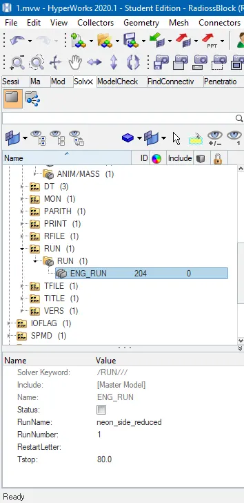
24. Edit the DT files under the Engine Keywords. Under the ANIME tab edit the ANIME/DT and set Tfreq to 0.5 as asked for the timestep. As per the recommendation, we can set the time step between 0.1 to 0.5ms and run time to 80ms. Now edit the ENG_RUN under the RUN tab and set Tstop as 80 ms.

Output Request

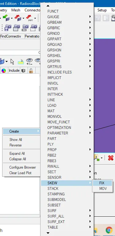
25. Now we will make necessary arrangements to meet our output request. The study of intrusions in the car cabin near the door will be done through skews. Right-click on the solver browser and select Skew with the FIX option. Select the three nodes to make up the local cartesian coordinates.

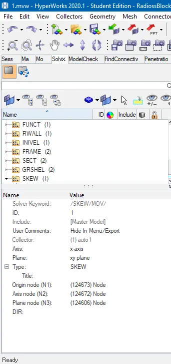
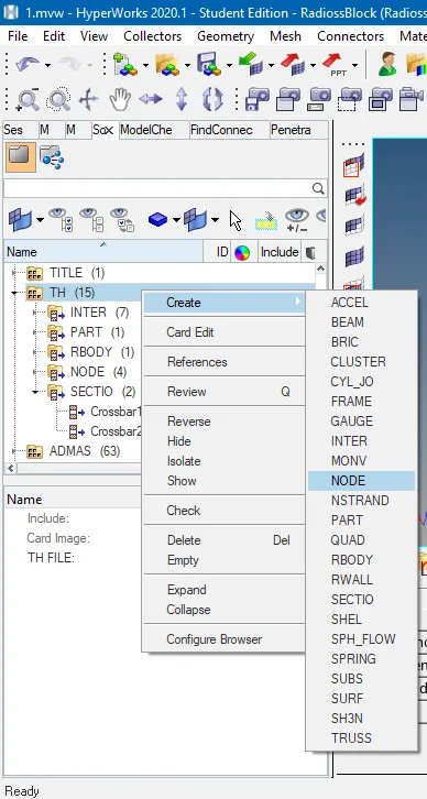
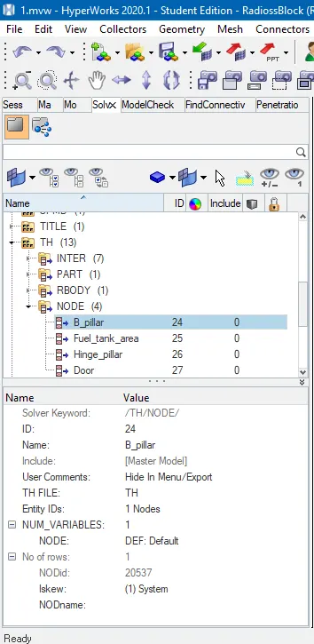
26. Create the /TH/NODE card under the solver browser and select the required nodes and then the fixed skew near the Right B-cabin pillar rocker support. There the travel of the node is computed from the global coordinates and it is presented In the local coordinates. The overall travel of the node is obtained.

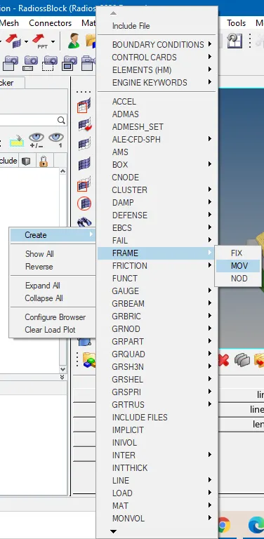
27. Let's create a moving frame for the section. To create a moving frame, Under the Solver deck, right-click to Create and then choose Frame with Mov option. Select the origin node, X-axis direction, and XY plane. This can be created based on the global coordinate system if possible based on the geometry orientation wrt global coordinate system.

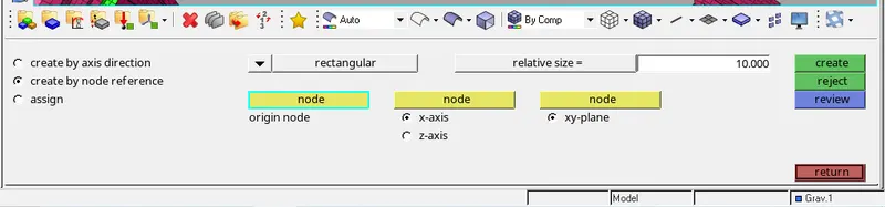
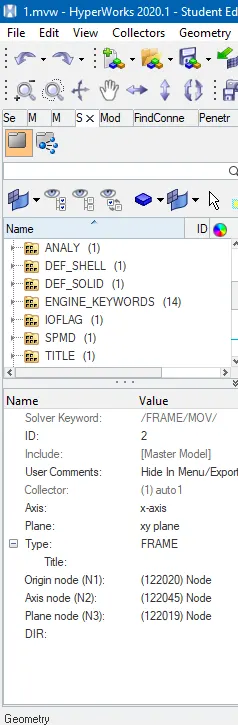
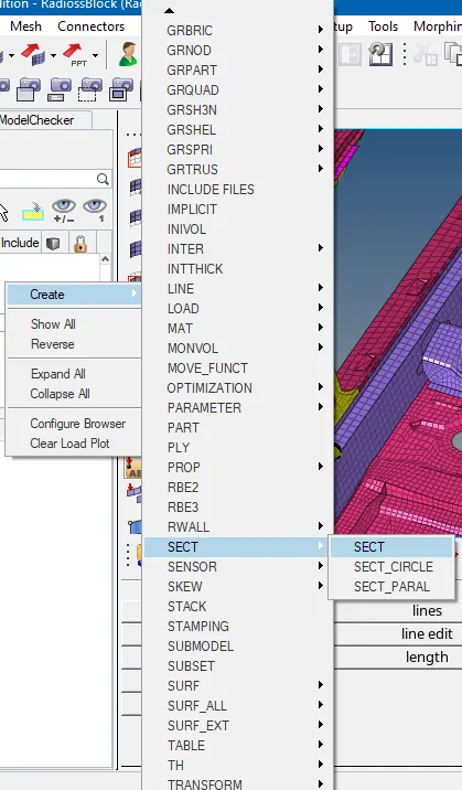
28. In the Solver browser, right-click and select the Sect Option. First, select the frame that is already created and assign it to the section. Select the required shell elements using the grshel_id option. Then Right-click to create in the new dialog box for required elements selection by clicking on the entity id as elements.

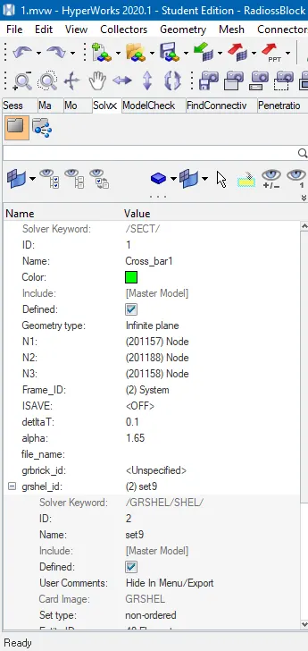
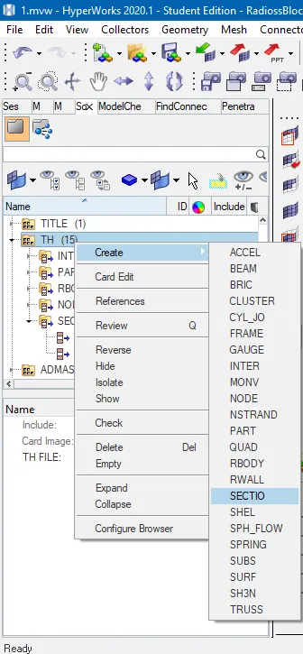
29. Enter the values for Isave as 2, deltaT as 0.1, and alpha with a default value of 1.65. Now to make a time history card, we can find the sectio option by right-clicking on the TH file under the Solve tab. Select the required cross-section.

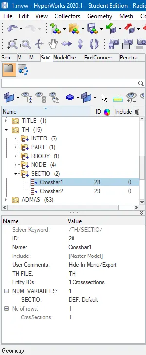
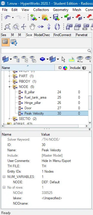
30. Inorder to record the peak velocity of the inner node of the door, create a time history card(TH/Node) for a node at the inner side of the door. Keep the skew_ID as global coordinates.

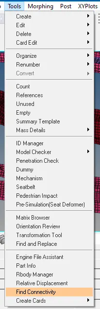
31. Check the connectivity of the model to root out any discrepancies. Select find the connectivity option under the Tools tab. Select components for Entities and include connectors for the check. We find out that three parts are free in nature and we will have to connect these three for a better simulation.

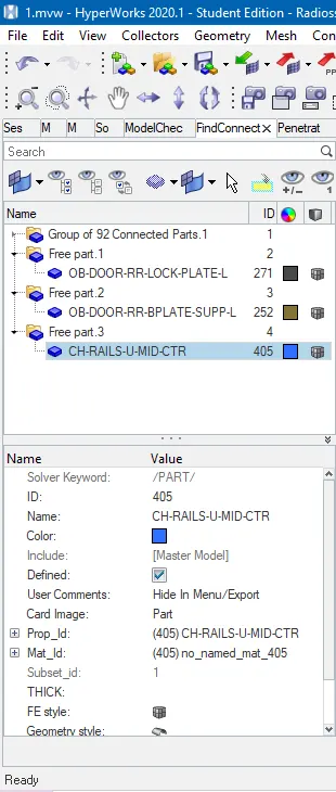
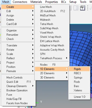
32. Create the simple RIGIDS to connect the free parts with the nearby components and use your personal judgment for the same Or you can leave the component as it since it is a scaled-down model of the original model and delete any free body.

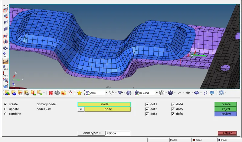
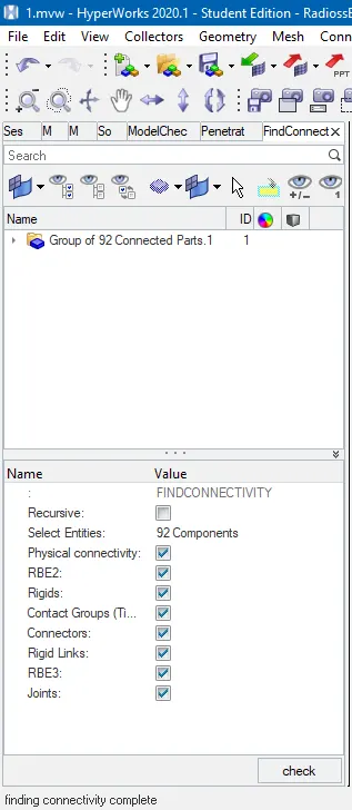
33. Run again after making the necessary changes and check again for connectivity error. No free part and just a connected group of 92 components.

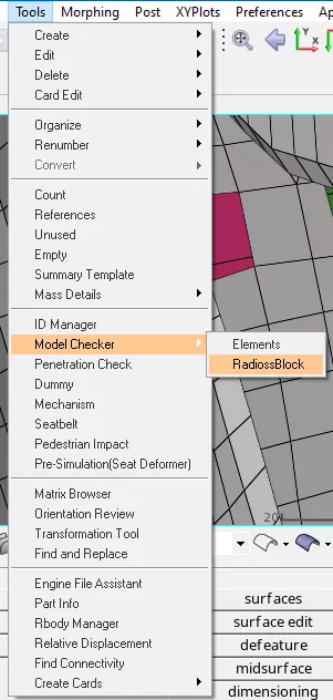
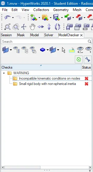
34. Finally, Run the Radioss model checker to see for any error. There should be no error and one can ignore the warnings. We should check for results to see if warnings are having any significant impact on the simulation. Select the model checker under the tools tab and then select the Radioss option. For both, the warning Incompatible kinematic conditions and a small rigid body won't have any significant effect on the model and hence we will ignore them. These warnings are the result of the scaled-down of the original model and their kinematics conditions.

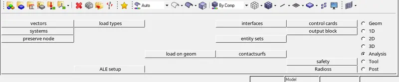
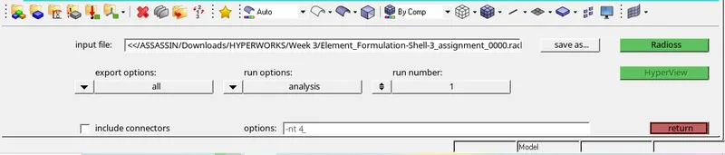
35. Go to the Analysis tab and run the radioss simulation. Select option for Export Option, Analysis for run options, and run number Should be 1. Also include the connectors for the analysis.

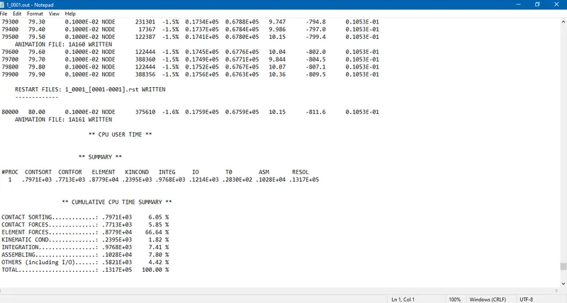
36. At the end of the simulation, do the energy error and mass error checks and determine whether the results would be acceptable. Since the Energy error% is around -0.9% and the Mass error at 0.029 we will go ahead and check the results.

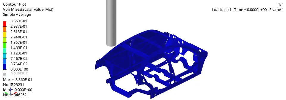
37. Open Hyperview and import the .h3d file to see the results such as Specific energy, plastic strain, and Von mises energy. Select the Contours under the plots which can be found in the result tab. Now select and result in type and its magnitude. For some results select the components and select simple in the case of the averaging method.

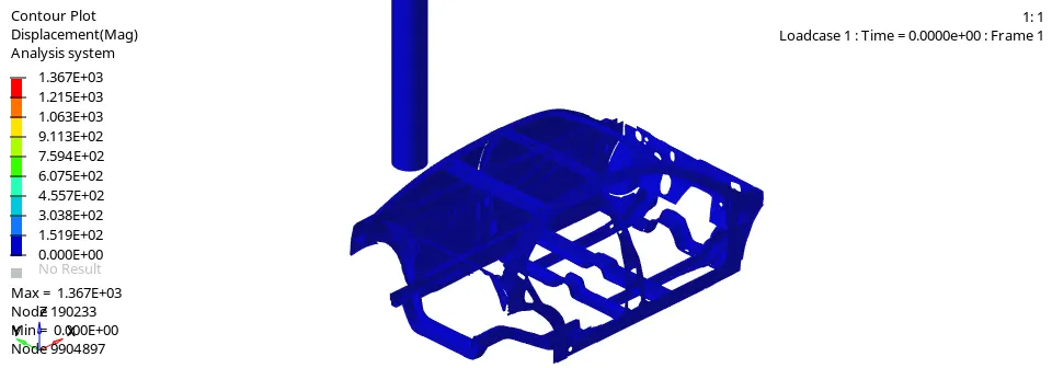
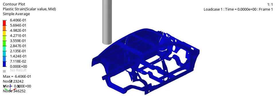
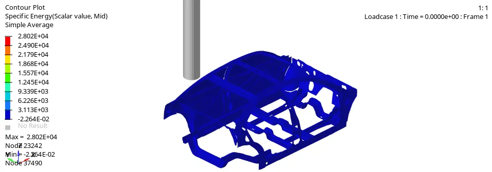
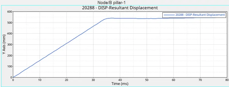
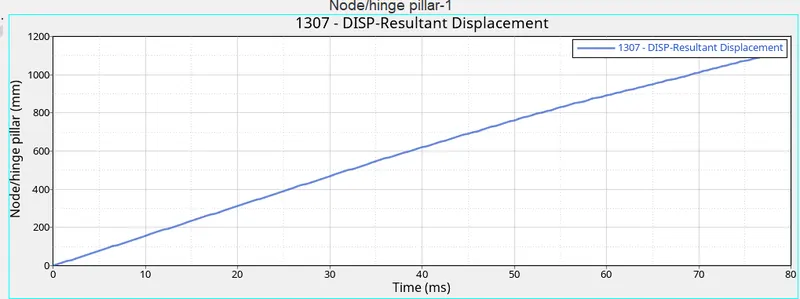
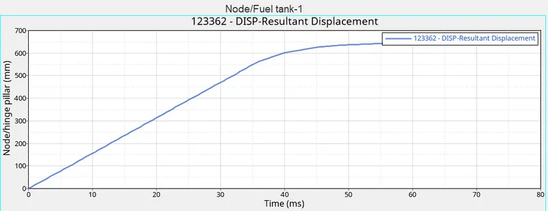
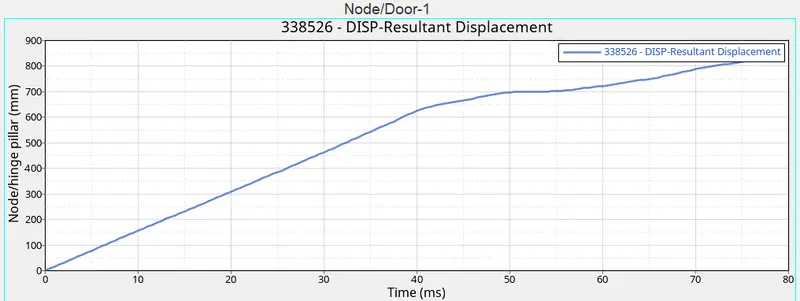
38. Open 2D Hyperview and plot 2D graphs. First, we will look for door intrusion after the crash. We have five node points which we will look into for results.

• B pillar

• Hinge pillar

• Fuel tank region

• The inner node of the door

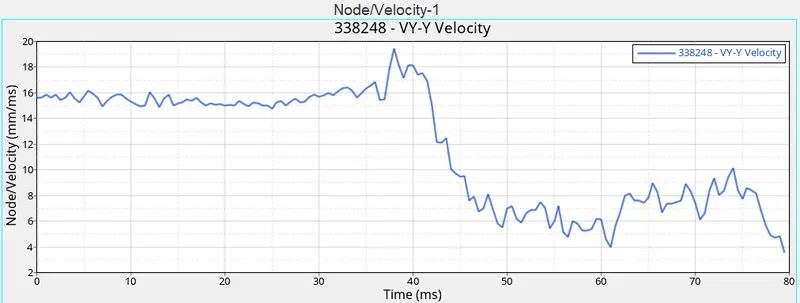
39. Now we look for the results for the peak velocity at the inner side of the door. We will evaluate the VY-Y Velocity as it will give us the peak velocity at the node since the body is transversing in the Y-axis to have the side impact.

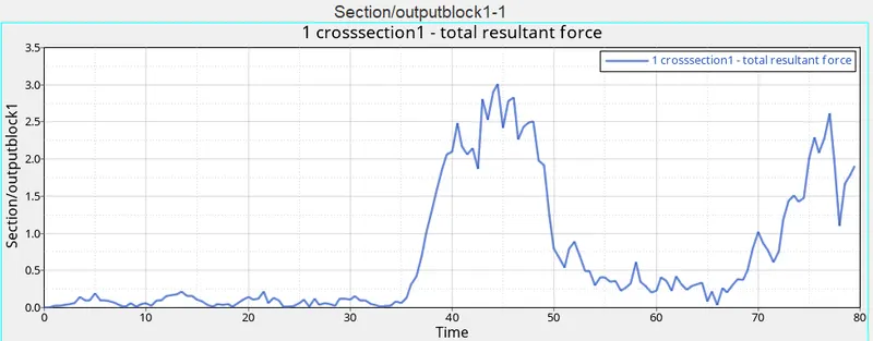
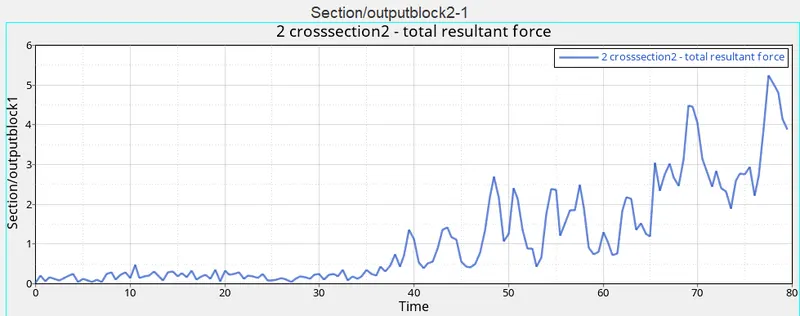
40. Now we will look for the forces on our crossbar sections created in the model.

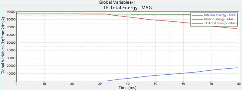
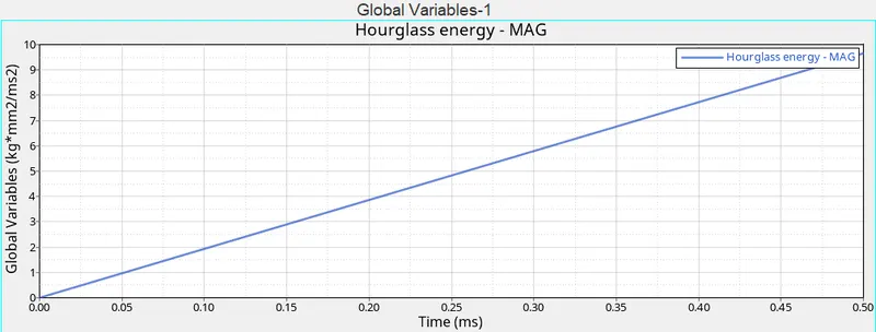
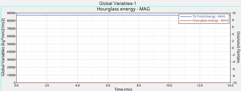
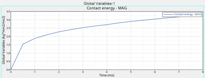
41. We will plot various energies to see how the body reacted upon getting in contact with the pillar.

• Internal Energy, Kinetic Energy, and Total Energy.

• Hourglass Energy.

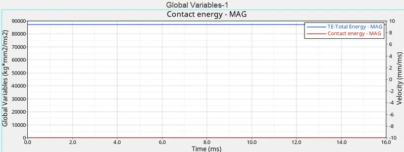
• Contact Energy.

RESULT

We saw a normal termination with no of the cycle of 80001 and elapsed time of 3805.77 s. We saw that the Energy error % is around -1.5% and the Mass error at 0.0105 and found them to be satisfactory.

We will note down the intrusion value inside the occupant's cabin with respect to the Right side B-pillar rocker support for each node's placement.

Nodes Placement	Intrusion (mm)
B pillar	540.07
Hinge pillar	908.62
Fuel tank region	646.47
The inner node of the door	730.20

We notice with the plots for the intrusion taking in the case of the Hinge pillar is the highest and follows a somewhat linear path. It has seen the majority of deformation compared to others. The least intrusion took place through B-pillar followed by the Fuel tank which is necessary to prevent any major damage to the tank.

The inner node at the door saw a peak velocity of 19.46 mm/ms approximately seconds after the impact taking place with the pole. Then velocity slowed dial down as kinetic energy gets converted into impact energy deforming the vehicle.

The side impact analysis was performed with the just the B-cabin of the BIW. Due to the limitation of Radioss solver to import the full BIW model with 300k element, we had to reduce the size to a bare minimum to continue the analysis. The mass of the BIW was initially was just 166 kgs which was increased to 700 kgs to intimate the whole car model with proper mass and CG.

The resultant force at the section of the front crossbar is around 3.006 Kgmm/ms2 and for the rear crossbar is 5.23 Kgmm/ms2. The front section area faced the initial brunt just as the impact took place but the rear section area confirms to have received major aftershock from the impact. The impact at the rear crossbar had a longer effect but the aftershock in the front crossbar tries to dial down for some time.

CONCLUSION

We have added mass on the nodes to get a value of CG to mimic the full model and the simulation will not be 100% the same as that of the real model. We cannot set up the miss parts properly and will present some errors for sure.

The hourglass and contact energy imparted in the simulation is very small when compared to the total energy imparted on the vehicle. Internal energy and Kinetic energy is the total sum of Energies. When Internal increases with the crash taking place and getting converted into kinetic energy it lead to the stable total energy. The Kinetic energy is highest before the crash takes place as the vehicle is moving at a certain speed. Just as the crash takes place kinetic energy starts it starts to dial down and get converted into internal energy.

The velocity imposed on the model is around 35 MPH which can be easily possible in the case of a head-on collision of the car with rest to the simulated vehicle.

The B-pillar saw the least intrusion and deformation as they are designed in such a way that they absorb most of the impact energy and bear the major shock. The occupant is kept safe as the result.

We can see that the resultant force value for the sections on both sides of the body has different values prompting us to conclude that the stiffness of the body is not symmetrical. Also if see the sectional force on rails, the right side it seems to have absorbed more impact force than the left side of the body even though the overall peak value is almost the same for both sides.

As far as the error is concerned we did not encounter any during the simulation but had some warning regarding the MATERIAL LAW1, rigid wall, and Interface gap in connection with the free bodies. They did not have any significant effect on our simulation. So we will ignore them for this analysis.

Finally, as far as the side crash simulation is concerned it is important for the BIW to absorb the energy and come to rest to prevent any major intrusion in the B cabin(Passenger seating zone). It is important for the safety of the occupants and that's why we measured the intrusion in the cabin space.