Meshing of a Bumper component and performing simulation of a Crash tube with different contact interface options. 

Objective

The meshing of a Bumper component and performing simulation of a Crash tube with different contact interface options.

Bumper Meshing

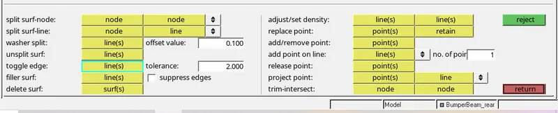
1. Clean the geometry and make sure the component is removed from free edges, etc. Use other tools available in the quick-edit panel to clean the geometry before generating the mesh.

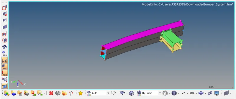
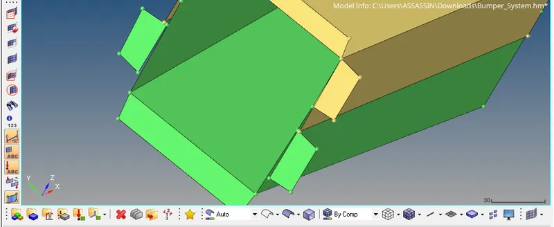
2. Mesh the model using automesh option under the 2D tab to get the elements. Keep the mesh type as quads only with an element size of 6mm.

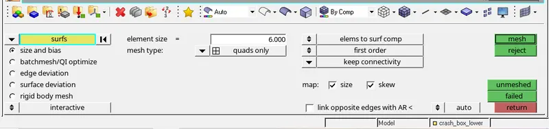
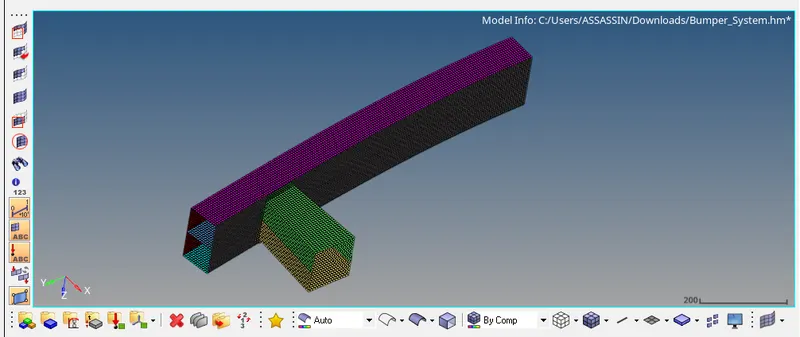
3. The current is only half of the original bumper and elements need to be reflected to get the full bumper component. Provide the appropriate 1D weld elements to the support arms of the bumper body.

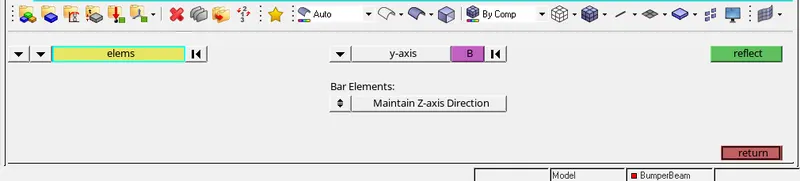
4. Duplicate the current element and assign it to the Bumperbeam component which is empty. Use the reflect option under the tool tab and reflect the element to the other half.

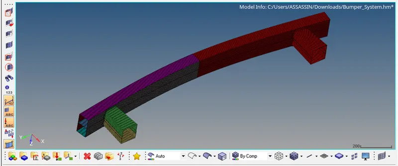
Impact Analysis of the Crash Tube

Procedure

Case 1

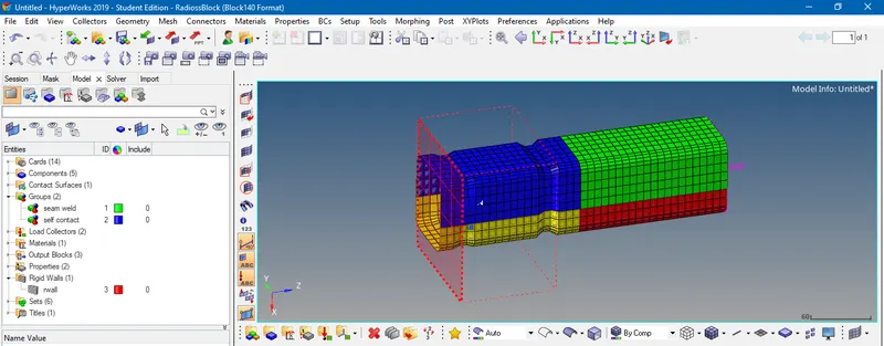
1. Import the .rad file using the solver deck option. Change the view from wireframe to shaded elements and mesh line, Also make the Rigid wall and rigid body visible in the solver. Create the TH stamps for all the parts along with the existing node, Rigid wall, and rigid body.

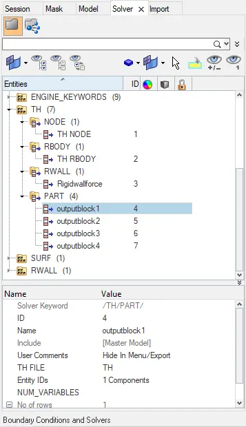
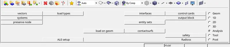
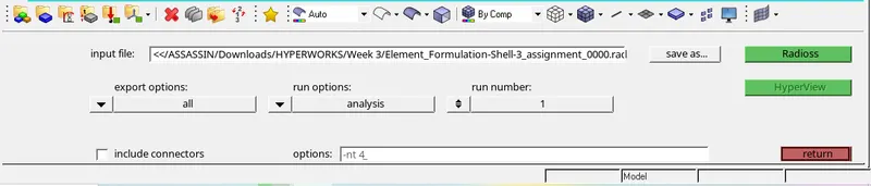
2. Run the base analysis without any modification to the properties. Select option for Export Option, Analysis for run options, and run number Should be 1.

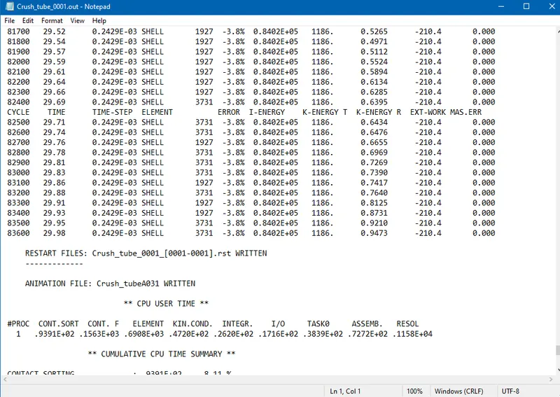
3. At the end of the simulation, do the energy error and mass error checks and determine whether the results would be acceptable. Since the Energy error% is around -3.8% and the Mass error at 0.0 we will go ahead and check the results.

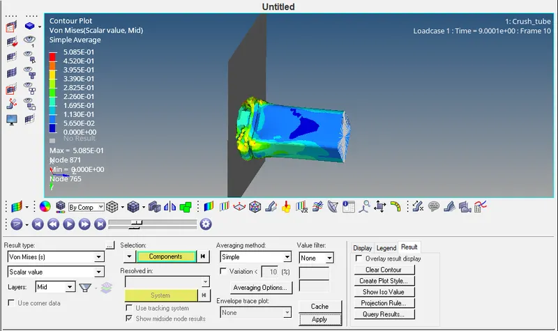
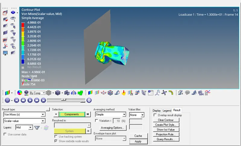
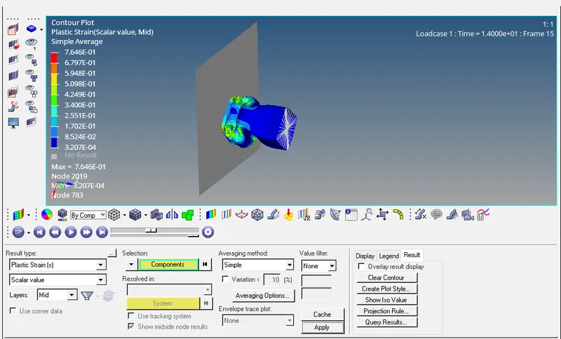
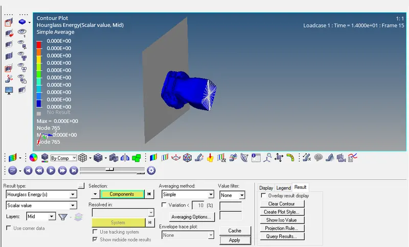
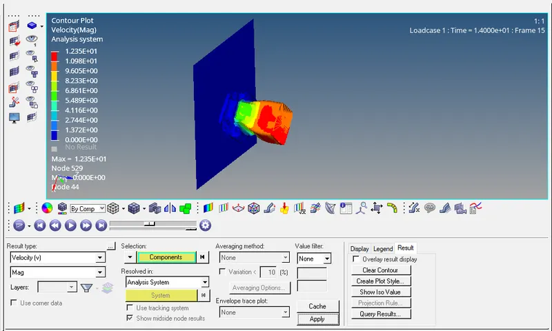
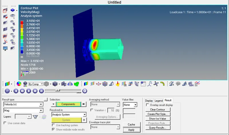
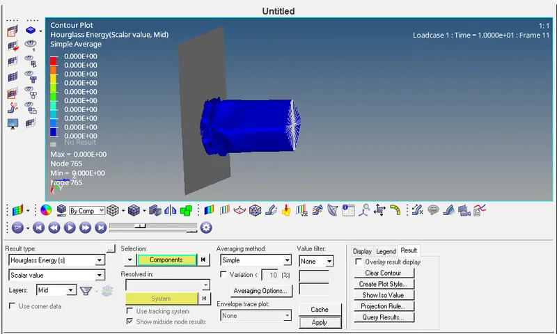
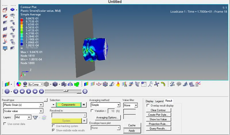
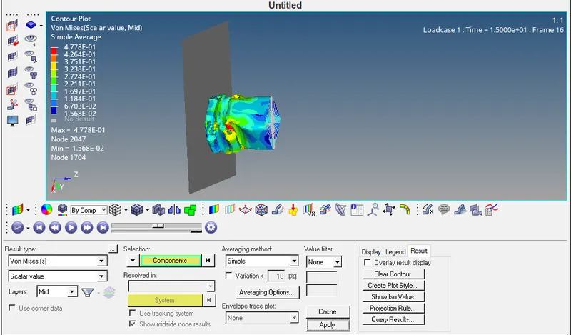
4. Open Hyperview and import the .h3d file to see the results such as velocity, Hourglass, plastic strain, and Von mises energy. Select the Contours under the plots which can be found in the result tab. Now select and result in type and its magnitude. For some results select the components and select simple in the case of the averaging method.

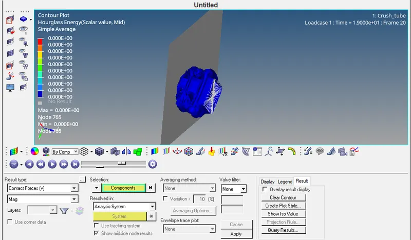
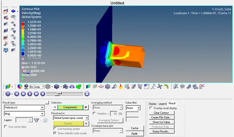
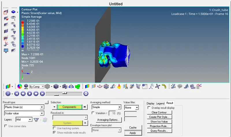
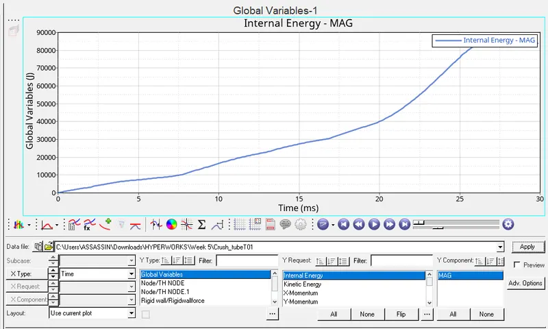
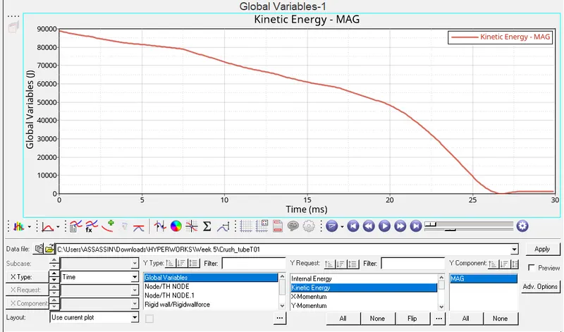
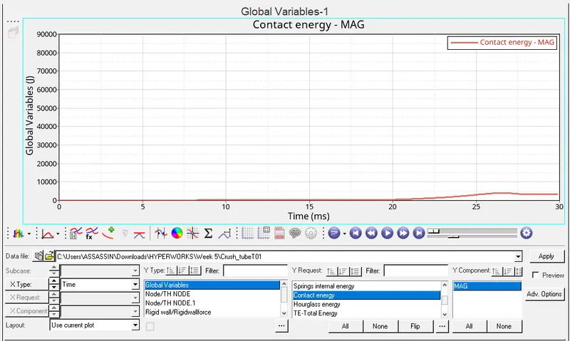
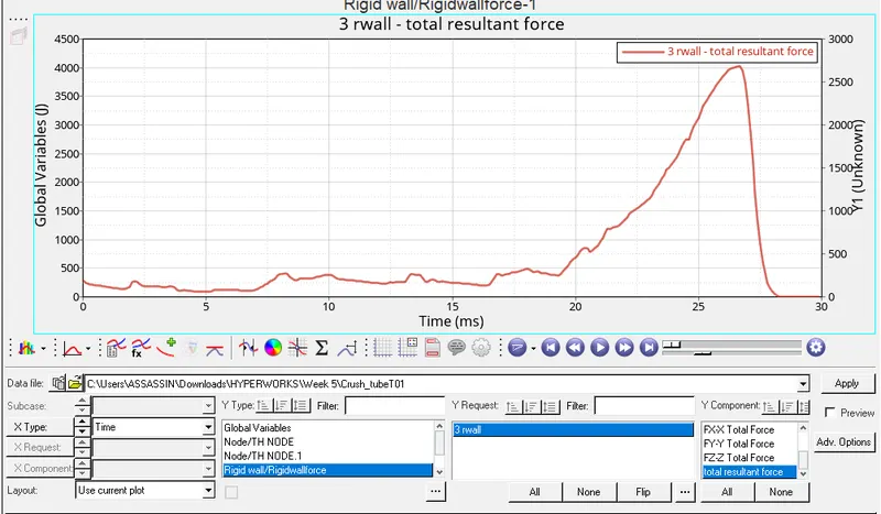
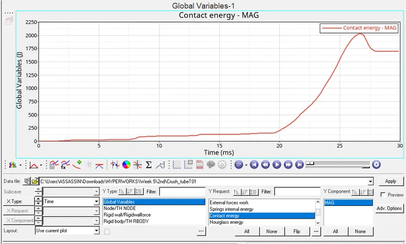
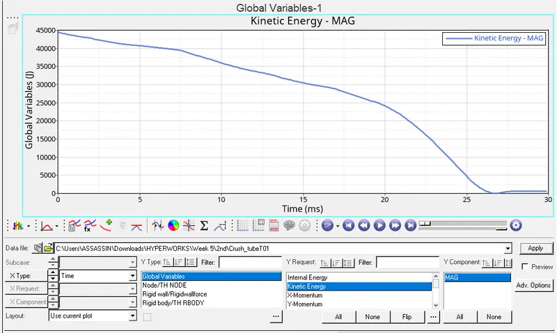
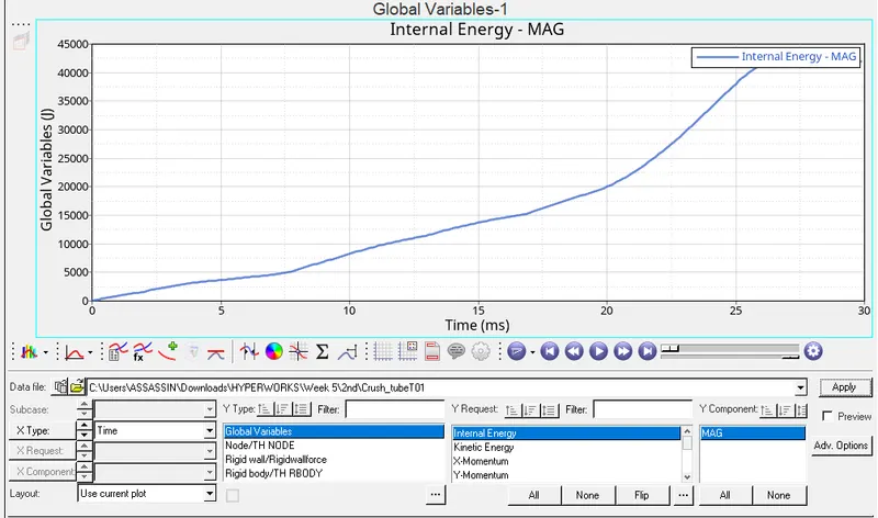
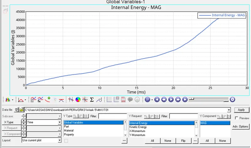
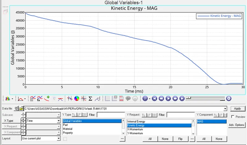
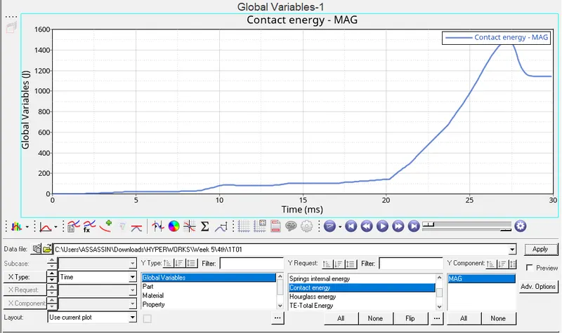
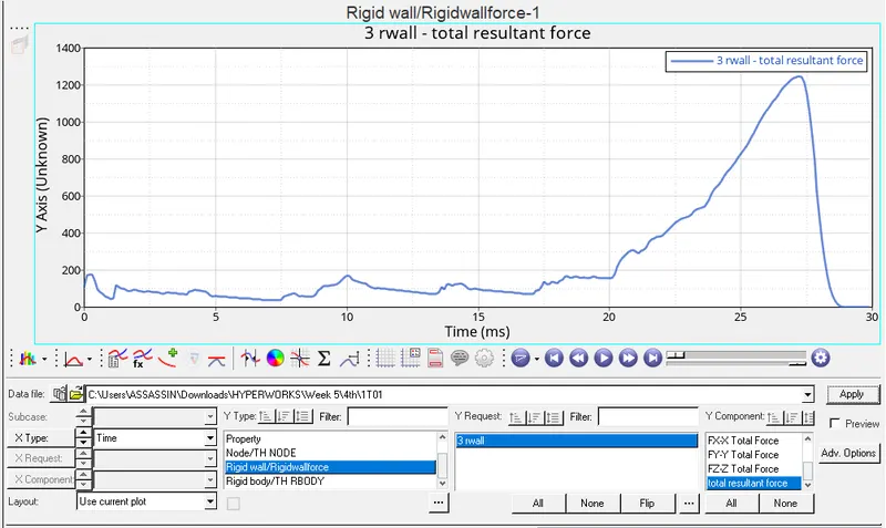
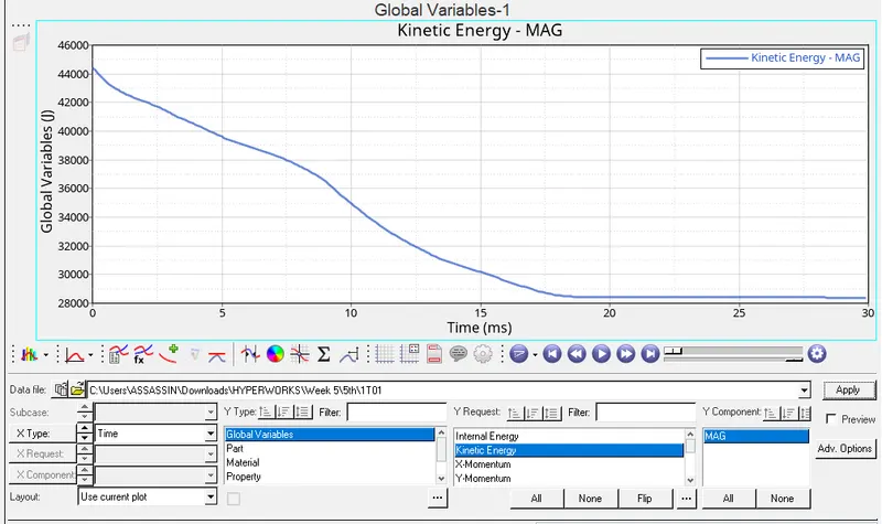
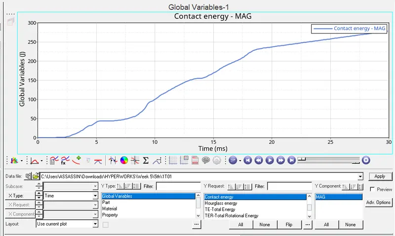
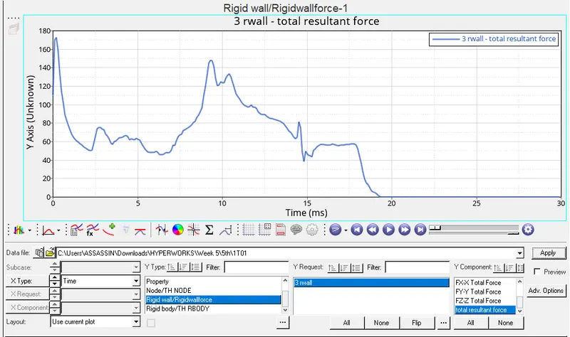
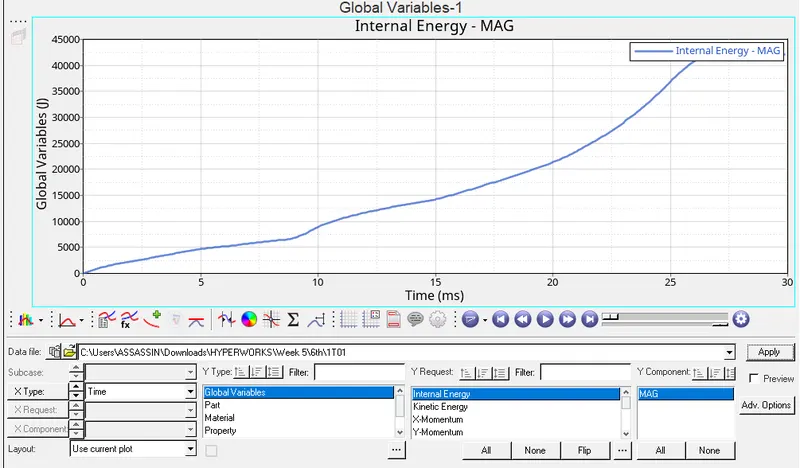
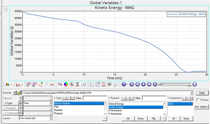
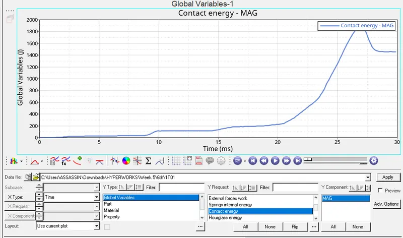
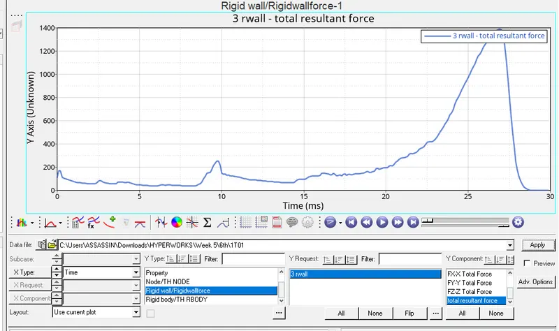
5. Open 2D Hyperview and plot 2D graphs for plots for kinetic forces, internal energy, contact energy, and Rwall forces.

Case 2

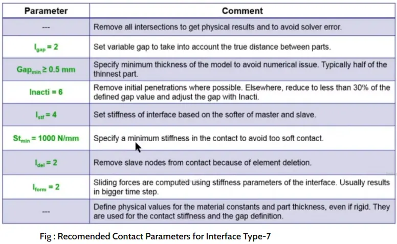
6. Open the .rad file in Radioss and Change the Inacti=6. We can find the same under the Contact interface tab in the Model Slab. We can only find the Inacti option in the Type 7 control interface. In this case, the initial penetration will be removed wherever possible or reduce to 30% of the defined gap and adjust the gap with Inacti.

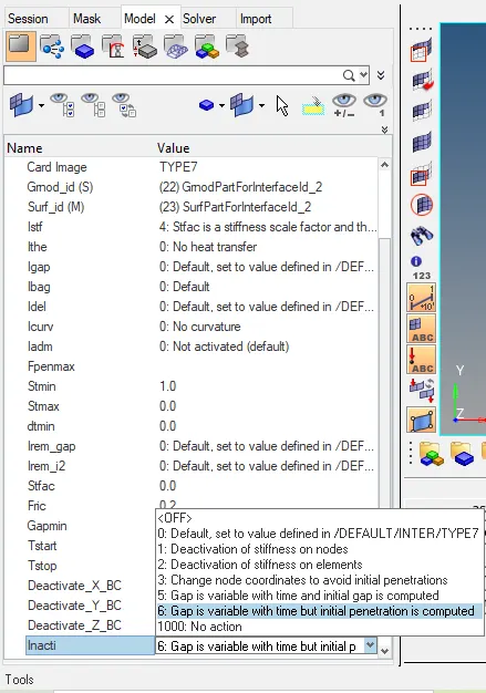
7. Save the changes and run the simulation. Open Hyperview and import the .h3d file to see the results such as velocity, Hourglass, plastic strain, and Von mises energy.

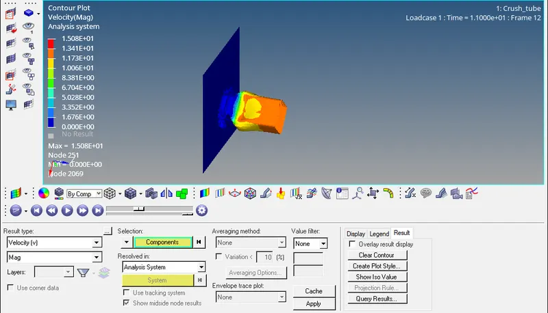
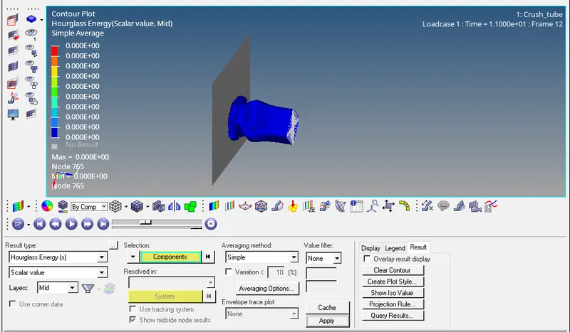
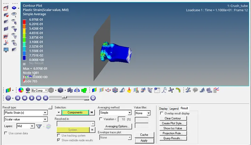
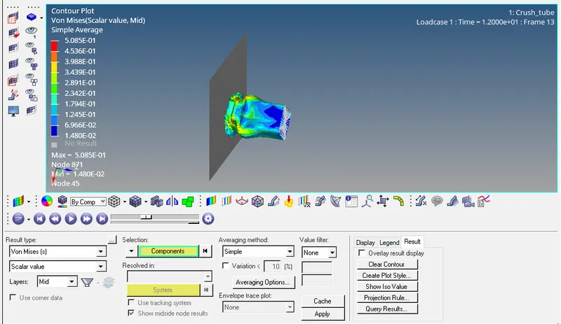
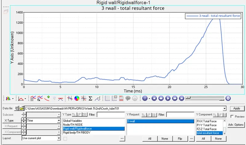
8. Open 2D Hyperview and plot 2D graphs for plots for kinetic forces, internal energy, contact energy, and Rwall forces.

Case 3

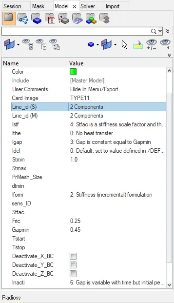
9. For case 3, create a new contact interface under the groups tab which is available under the model deck. Select the slave line and master line taking into account that slave nodes will not penetrate the master surface. Rigid surfaces must always act as Master surfaces and node-based surfaces can act only as Slave surfaces.

10. Save the changes and run the simulation. Open Hyperview and import the .h3d file to see the results such as velocity, Hourglass, plastic strain, and Von mises energy.

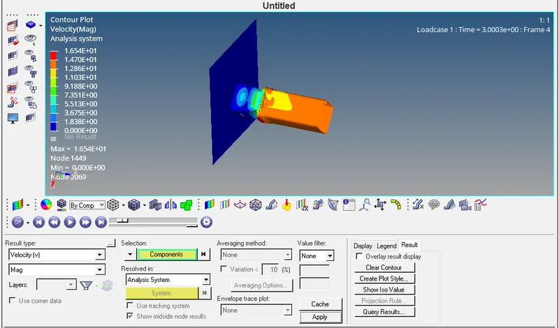
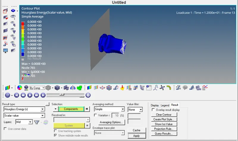
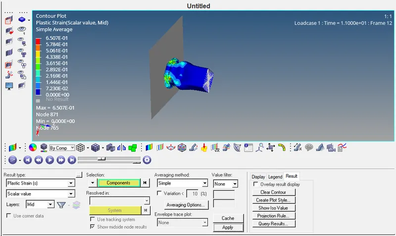
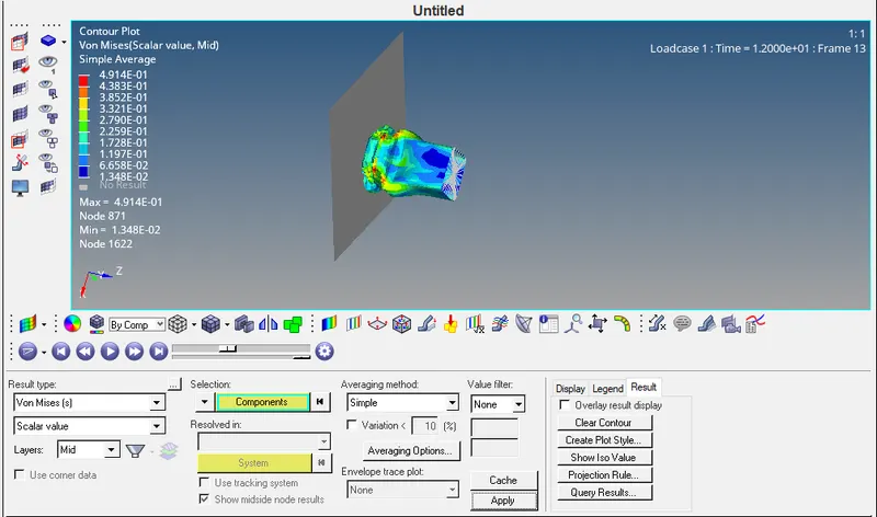
11. Open 2D Hyperview and plot 2D graphs for plots for kinetic forces, internal energy, contact energy, and Rwall forces.

Case 4

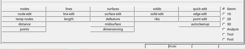
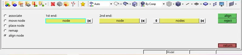
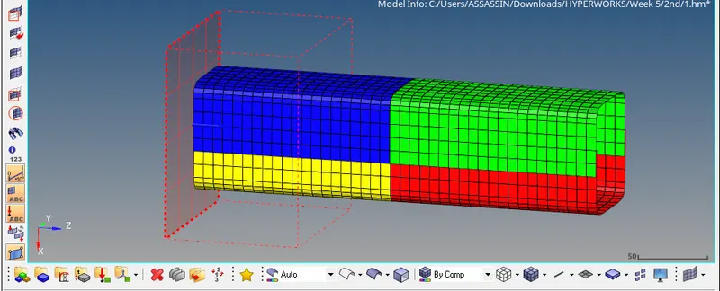
12. For case 4, we will remove both notches and remove boundary conditions on a rigid body. In order to remove the notches, go to the geometry option and select the node edit option from it. Select the align node option and remove both the notches.

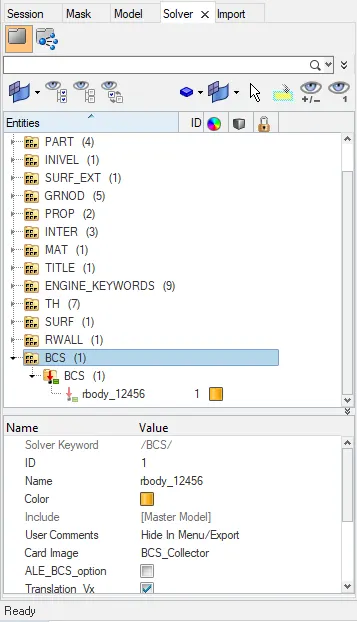
13. Remove the boundary conditions by deleting the BCS option under the solver tab. Save the changes and run the simulation.

14. Open Hyperview and import the .h3d file to see the results such as velocity, Hourglass, plastic strain, and Von mises energy.

15. Open 2D Hyperview and plot 2D graphs for plots for kinetic forces, internal energy, contact energy, and Rwall forces.

Case 5

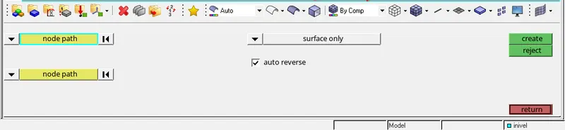
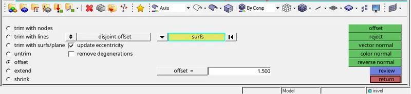
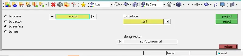
16. Create a new surface in the middle of the section using the ruled option available in the 2D tab. Then press Shift+F9 to get the offset dialog box and do the surface offset of 1.5mm. Finally, project the nodes from the middle of the section to create a notch. Select the path line for the nodes, select the surface and use it along the vector as a surface normal.

17. Save the changes and run the simulation. Open Hyperview and import the .h3d file to see the results such as velocity, Hourglass, plastic strain, and Von mises energy.

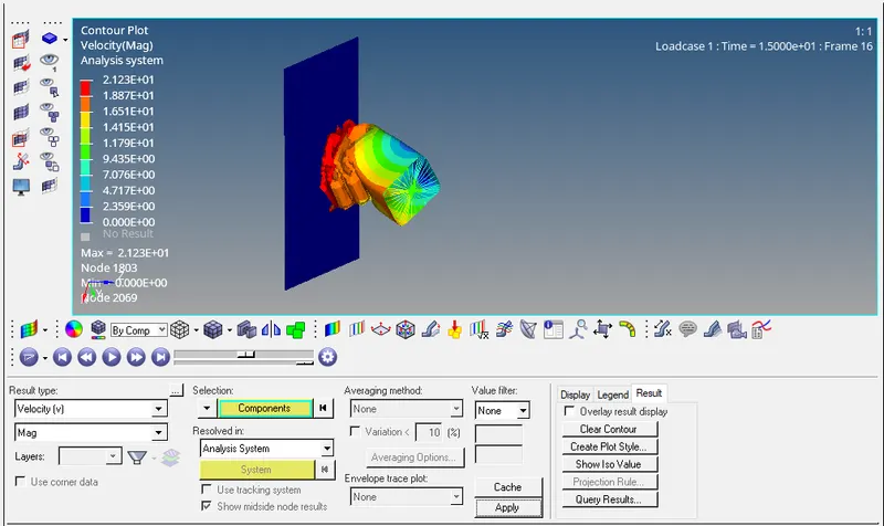
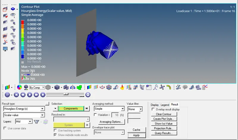
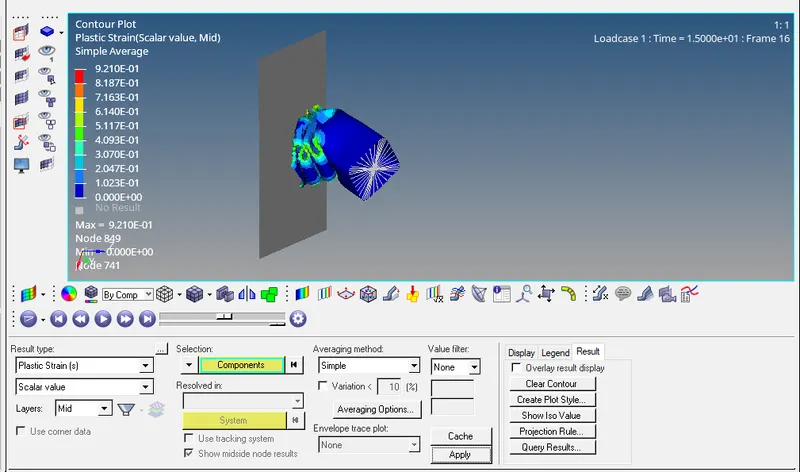
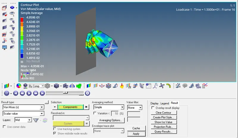
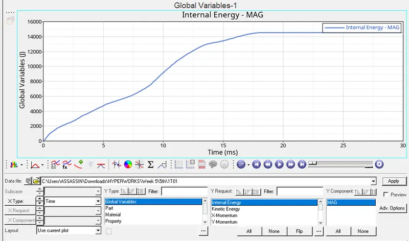
18. Open 2D Hyperview and plot 2D graphs for plots for kinetic forces, internal energy, contact energy, and Rwall forces.

Case 6

19. Follow the above-mentioned procedure to create the notch on the opposite side of the section.

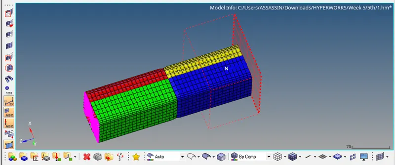
20. Save the changes and run the simulation. Open Hyperview and import the .h3d file to see the results such as velocity, Hourglass, plastic strain, and Von mises energy.

21. Open 2D Hyperview and plot 2D graphs for plots for kinetic forces, internal energy, contact energy, and Rwall forces.

Result

Cases	Plastic Strain	Von Mises	Rwall Forces	Contact Forces	Internal Energy(J)	No of cycle	Simulation time (s)
Case Study 1	1.204E+00	6.964E-01	2681.318	4063.191	84539.484	83691	359.40
Case Study 2	1.204E+00	5.879E-01	1340.659	2031.595	42269.742	83691	178.18
Case Study 3	1.111E+00	6.110E-01	1351.526	2182.930	42141.203	83174	208.92
Case Study 4	1.356E+00	6.679E-01	1245.304	1493.794	42700.097	76983	215.21
Case Study 5	9.210E-01	4.677E-01	172.880	278.213	14517.27	83814	184.06
Case Study 6	1.257E+00	6.488E-01	1389.117	1887.145	42360.238	91537	231.65

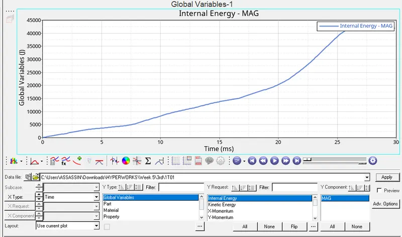
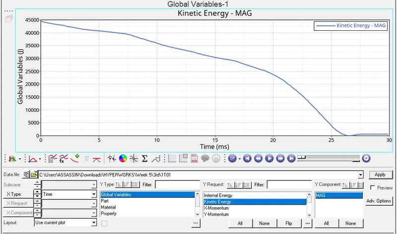
Internal energy and Kinetic energy is the total sum of Energies. When Internal increases with the crash taking place and getting converted into kinetic energy it leads to the stable total energy. But after reaching the limiting strain rate it leads to some resistance force leading to an increase in kinetic energy making total energy unstable.

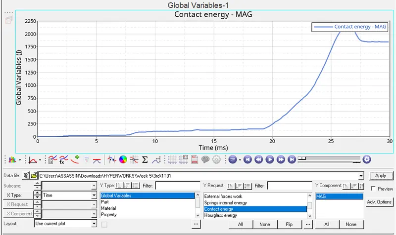
Contact energy is a combination of contact force (b/w master and slave node) and penetration. When a crash takes place, the contact force is the force applied (b/w master and slave node), and energy resisting to overcome the penetration between the slave and master.

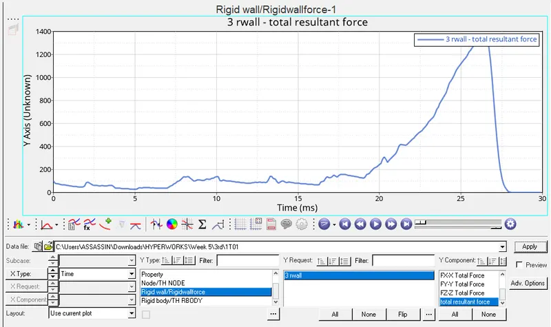
Rigid wall force is created at the point of contact between the rigid body and the crash tube. When reaching the peak strain rate, we see a sudden drop of the rigid wall due to a decrease in the impact intensity.

For case 1, the base file was run without any changes. This is a base simulation used for the template values for the case study.

In case 2, we change the Inacti=6 and run. The initial penetration will be removed wherever possible or reduce to 30% of the defined gap and adjust the gap with Inacti. This leads to a decrease in simulation time, Rwall force, contact energy, etc due to the removal of any initial penetration.

For case 3, we are using the type 11 contact interface with the recommended properties. It stimulates impact edge to edge or lines(beam, truss, or other 1D elements). It increases the computational time without any significant change in the energy and a small reduction in the number of cycles.

For case 4, we are removing up both the notches, and smooth plain model geometry is generated. We have also removed the associated boundary conditions on the rigid body. In prior cases, we can observe the deformation taking place at the notches initially, and then the whole of the tube gets compressed. No significant change in the energy.

In case 5, we see that a single notch that is leading the deformation leads to an abrupt end as the crash tube flips over and the body is unstable due to the loss of constraints on DOF by the boundary conditions. A significant reduction in energy.

For case 5, we see better stability to the model with the introduction of the opposite notch. Internal energy, plastic strain, and von mises are somewhat the same as case 4 but a significant increase in the contact energy. Increase in simulation time and number of cycle as compared to the previous case model.

Conclusion

Cases	Remark
Case Study 1	Run the crash tube model
Case Study 2	Change the Inacti=6 and run. The initial penetration will be removed wherever possible or reduce to 30% of the defined gap and adjust the gap with Inacti.
Case Study 3	Create the type 11 contact and run. Increase in simulation time but better capturing of the physical model.
Case Study 4	Remove both notches and remove boundary condition on rigid body node. Notch acts as a guide.
Case Study 5	Create a new notch in the middle. An abrupt end to analysis due to unstable model.
Case Study 6	Create a new notch with nodes only from opposing 2 faces

It is recommended to remove any initial penetration in the model which leads to an increase in contact energy, Internal energy, etc.

Type 2 and type 7 contact interfaces sometimes do not notice node to surface contact due to edges crossing each other at an angle. Type 11 interface allows self impact and should be used in specific cases. In the case of edge crossing, the Type 11 interface allows capturing the physical modal correctly.

Notches are guiding on how deformation will take place. Boundary conditions are necessary for a stable model during analysis as it brings in proper DOF constraints as in the physical world.

Optional way to edit the contact card in hypercrash

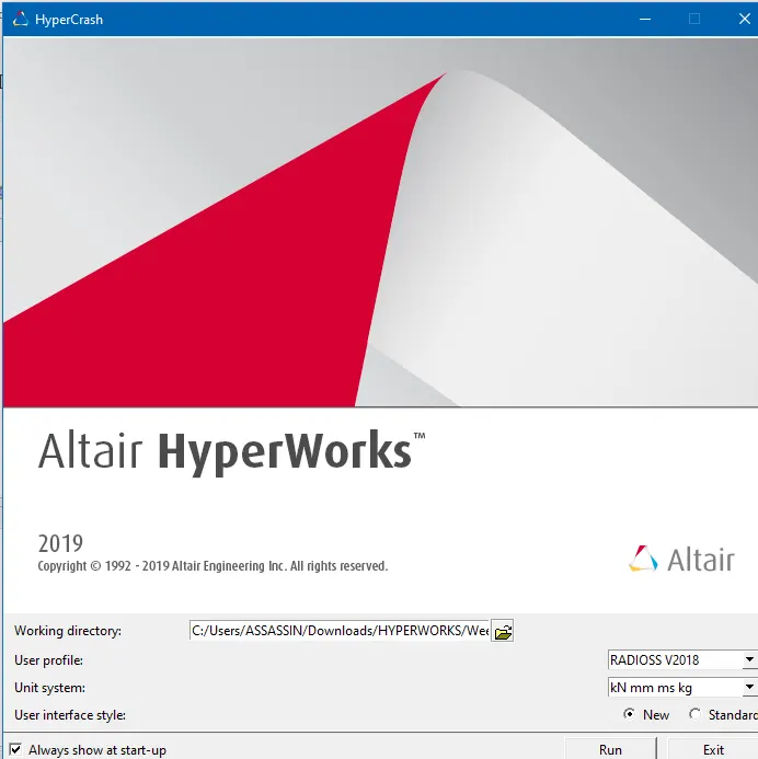
Open Hyperworks and select the Hypercrash option available in the Application drop-down menu. Select the user profile, file path, and finally uint system as kN mm ms kg.

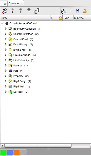
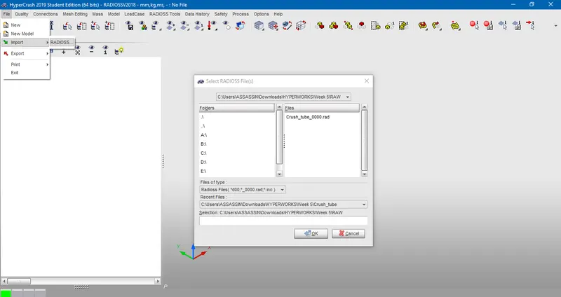
2. Import the .rad file in the Hypercrash application. Select the file path and import the crash_tube_0000.rad. You can see the entity tree and we can observe the entities like properties, material, etc.

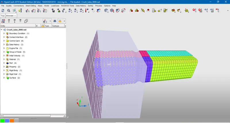
3. For this case study, we don't need to do any changes to the file. Export the file in radioss format and select the file directory and save the file for radioss. Hypercrash is used to make some necessary in the rad file which has to undergo the impact simulation.

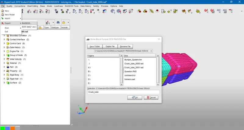
4. We can control the mesh element penetration, gaps, etc in hypercrash. We modify any irregular mesh profile, check the contact interface and provide initial velocity. Adding load cases, mass properties, material property, control cards, and even rigid body in case we want to overall simulation load.