Assignment 7

Q1) Explore tutorial number 9 and write a detailed report

Fast Running Engine Models are dynamic, fully-physical engine models that are designed specifically to run fast. While high-fidelity engine models are commonplace in the engine performance department, they are often too slow running to incorporate into system-level models where long transient events may be simulated, or where the simulation model must respond faster than real-time, such as for HiL (Hardware-in-the-Loop) simulations.

When simulation speed is of priority, high-fidelity GT-POWER engine models can be simplified into FRMs using a standard conversion process.

FRMs are able to achieve such fast run times by two means:

(i) increasing the simulation time step size, and

(ii) decreasing the number of calculations per time step.

These two means are often accomplished at the same time by lumping various flow volumes together which will reduce the total number of subvolumes and also allow for a larger time step size by increasing the effective subvolume length.

Example 9 is a 4cylinder SI-direct injection engine with a wastegate turbocharger.

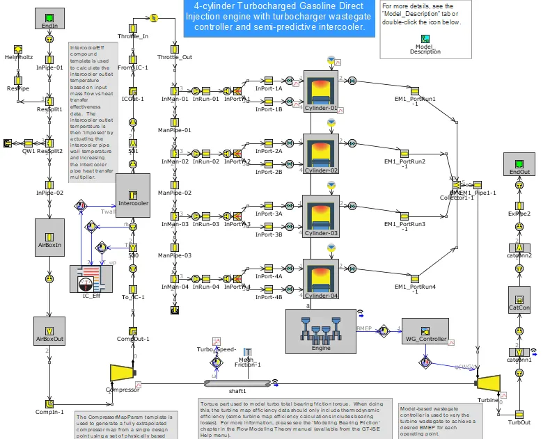
Run setup:

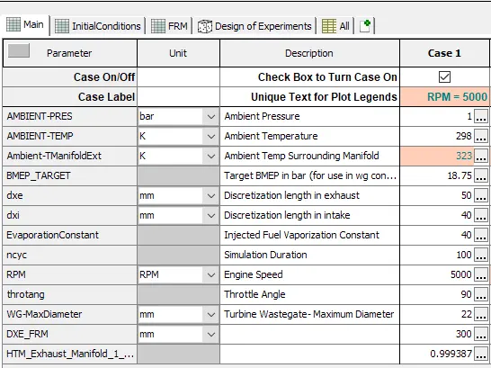
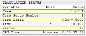
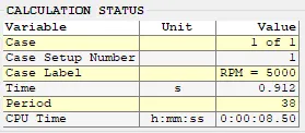
Time-taken for solving the solution: 38sec.

Converting the Full detailed model into FRM model:

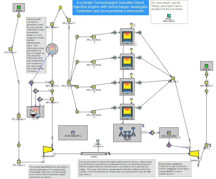
Here the control volumes at inlet and exhaust have been made as two volumes instead of discretizing it. Also instead of solving for all the cylinders, we will consider only one cylinder as a master cylinder (cylinder slaving), and its values will be given to all other cylinders.

Parts	Detailed model	FRM model
Turbocharger	The compressor and turbine part references a map file from which map data is read.	The CompressorMapParam and TurbineMapParam template is used to generate a fully extrapolated compressor map from a single design point using a set of physically-based parametric equations.
The Intercooler	It is modeled using a pipe part. The multiple pipes attribute is used to model a bundle of 100 identical pipes of 5.0 mm diameter each. The wall temperature is imposed at the desired outlet air temperature. An RLT Dependence object is used to make the imposed wall temperature (and thus the outlet air temperature) dependent on speed and load.	The IntercoolerEff compound is used to calculate the intercooler outlet temperature based on input mass flow vs effectiveness data. The intercooler outlet temperature is then 'imposed' by actuating the wall temperature and increasing the intercooler pipe heat transfer multiplier.

run setup:

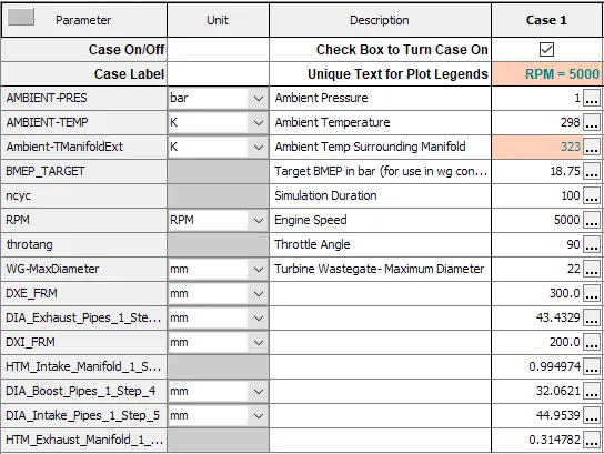
Time-taken for solving the solution: 8sec.

We can see a huge difference in the time taken to solve the model in FRM.

Comparison of Courant numbers:

The Courant number in one-dimension is defined as C ≡ u∆t ∆x where u is the characteristic wave speed of the system, ∆t is the time-step of the numerical model, and ∆x is the spacing of the grid in the numerical model.

Thus we can see, that if we reduce the number of subvolumes and the time step we can regulate the courant number and so the speed of simulation.

The lower the value of the courant number, the more likely the part will limit the timestep. This enables the user to determine multiple parts that will limit the timestep.

Thus by seeing the courant value for each part we can combine the parts which consume more time, together.

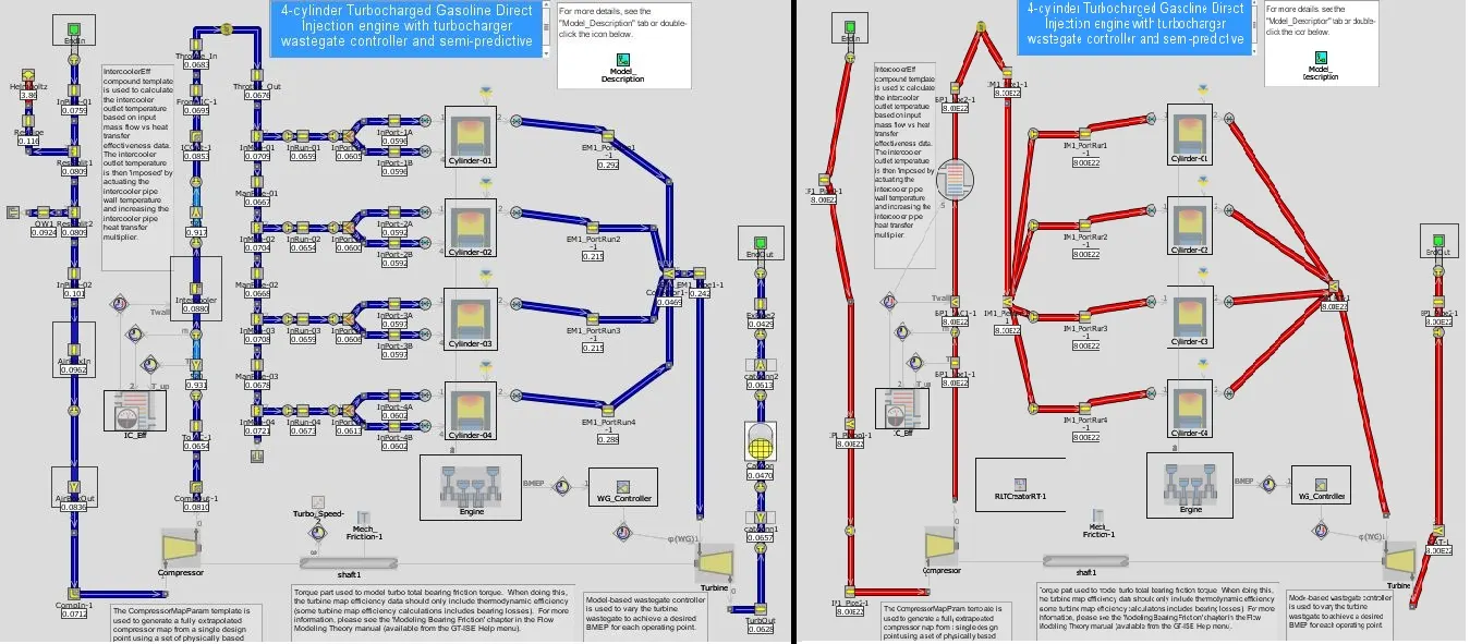
We can see from the model above, in the actual model the courant for each subvolume is defined and time for simulation also. This compared to the FRM model is less, where we have used fewer control volumes and timesteps.

Q2) Build FRM Model for the following configuration using the FRM builder approach

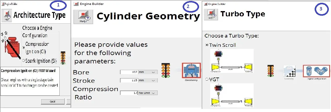
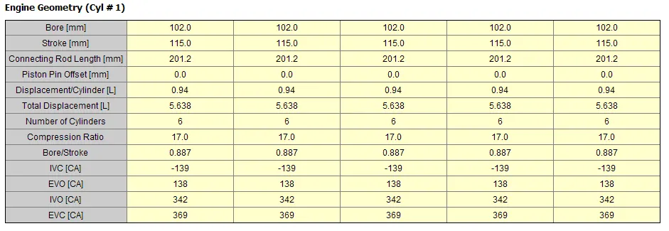
• Bore 102 mm stroke 115 mm CR 17
• No of cylinder 6
• CI engine
• Twin Scroll Turbine
• GT Controller
• Run all cases

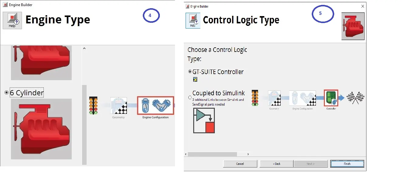
FRM builder procedure:

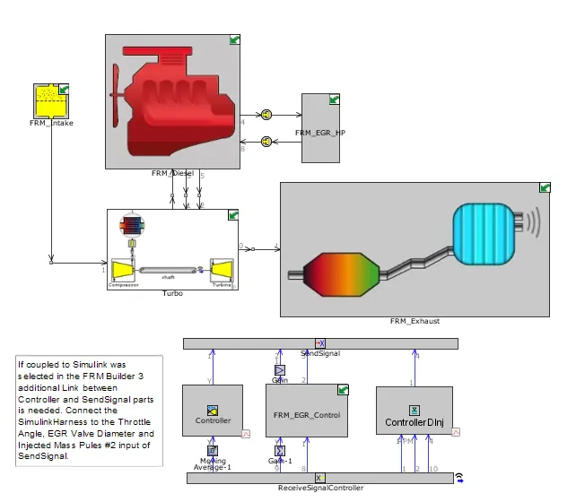
Final Model:

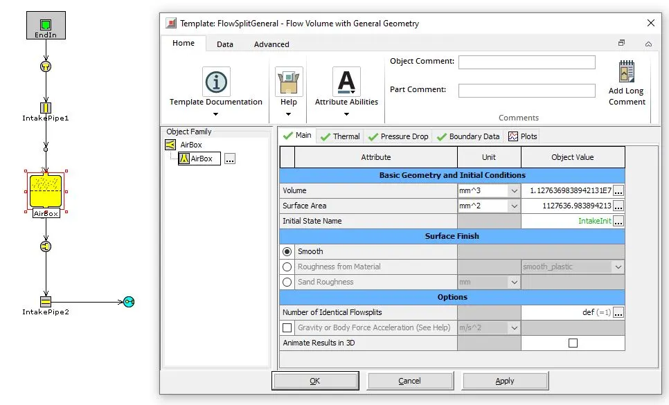
Intake system:

Exhaust system:

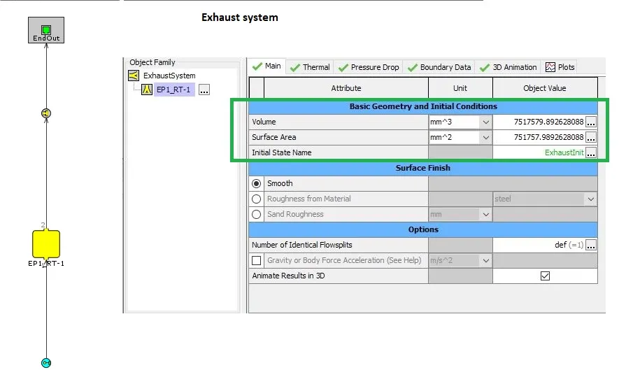
The FRM modeler has combined the series of connections at inlet and exhaust systems into a single volume.

Engine model:

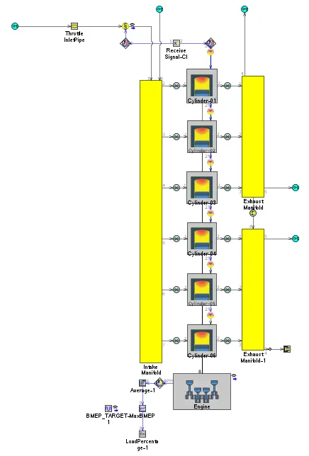
Here also the whole engine model has been made simple by using single large control volumes at the inlet and outlet. Since it is a twin-scroll turbocharger, we have two volumes present.

GT Controllers:

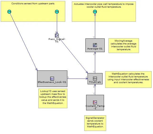
These controllers help to control the desired output value, by taking inputs from the input data and boundary conditions assigned.

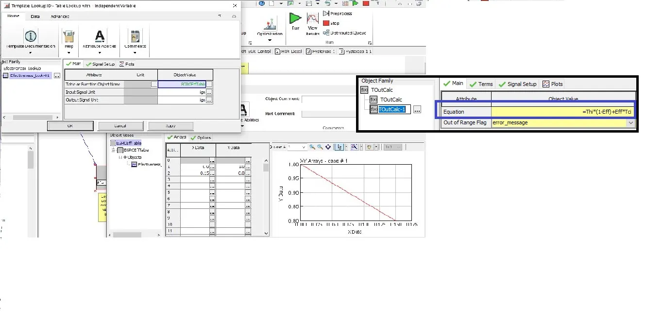
Here in the EGR effectiveness controller, we define the effectiveness as a function of rpm. The coolant temperature will be defined. Thus with the help of these values and a feedback system, the controller will calculate the desired effectiveness of the cooler.

Main controller:

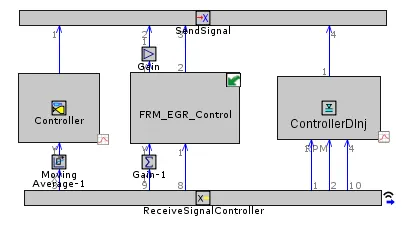
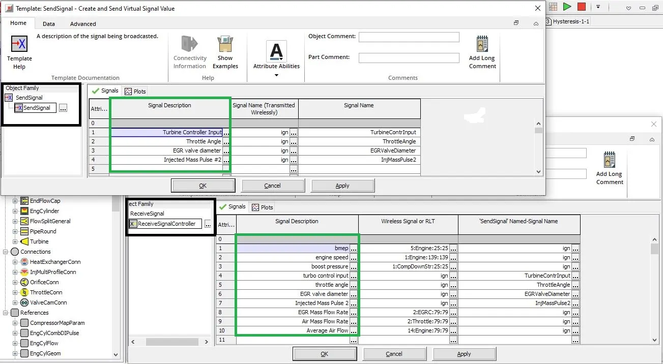
The above controller controls all the parameters associated with the engine, like the rate of fueling, EGR mass flow, coolant flow, etc so as to give the desired output values. The feedback system helps in maintaining the loop closed. The signals are wirelessly connected to each part so that the model layout does not become clumsy.

Each receiving and sending signals are numbered for easy understanding in the controller.

Results:

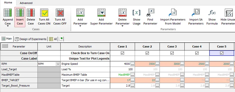
Case setup:

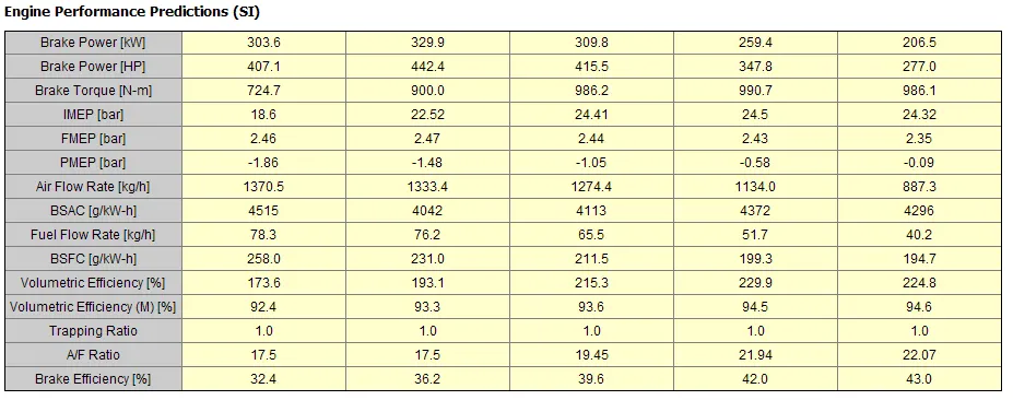
The BSFC value of the engine at 4000 rpm is high at 258, due to reduced air-fuel ratio.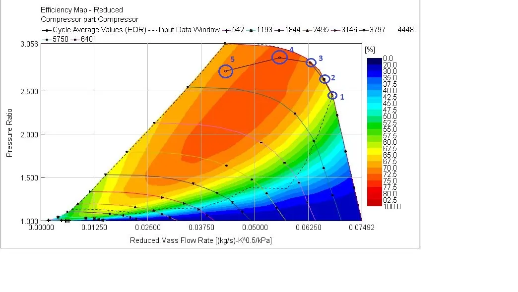

From the compressor efficency map we can infer that the point 1,2,and 3 are in the excess rotor region, and working in those region is not suitable for the compressor as it can cause mechanical damage to the blades.

Thus we can either go for a larger turbocharger or we can reduce the working speed of the compressor.