Frontal Crash Simulation of Vehicle Structure using Radioss

OBJECTIVE

1. To check the unit system and either follow [Mg mm s] or [Kg mm ms].
2. To create the appropriate interface, friction 0.2, and recommended parameters.
3. To make sure there is no penetration and intersection.
4. To correct issues related to rigid bodies, if any present.
5. To create a rigid wall with friction 0.1.
6. To compare the model weight with the full scale 300K nodes and use added masses to reach target weight 700 kg while getting CG about the required range.
7. To provide an initial velocity of 35 mph.
8. To use the model checker to ensure good quality
9. To assign min. time-step: 0.5 to 0.1 microseconds.
10. To run the simulation for 80 ms.

• Output Requests

1. Sectional force in the rails at the location of indicated node 174247.
2. The axial force received on the rails from the bumper.
3. Shotgun cross-sectional forces.
4. A pillar cross-section.
5. Acceleration curve received on the accelerometer at base B pillar (on B pillar rocker).
6. Intrusions on the dash wall 66695, 66244.

PRE-PROCESSING

The first objective of the challenge was to check the unit system. Fig. 1 shows the cad model of the bumper. From fig. 1, and fig. 2, it is certain that the [Kg mm ms] unit system has been followed.

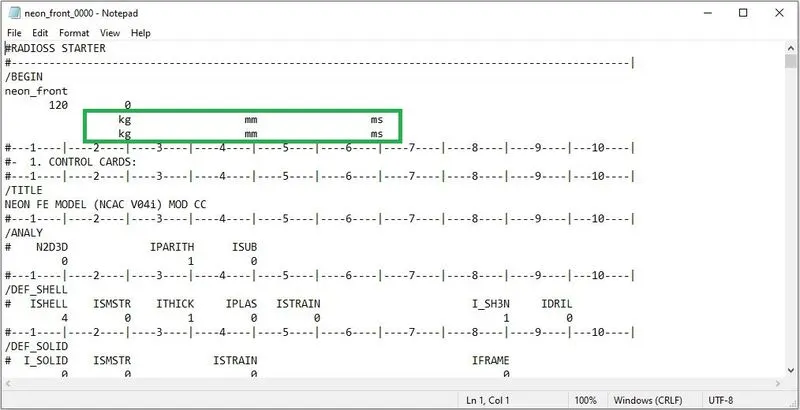
Figure 1: Unit system mentioned in starter file.

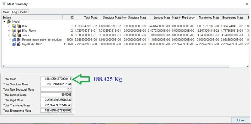
Figure 2: Mass summary of vehicle, mentioning it as188.425 Kg.

In material property, the E value is equal to 210. That must be in GPa or kN/mm². The density value is equal to 7.89e-06, which must be in kN/mm³.

The total mass of a vehicle is generally measured in tonnes. However, because of the software limitation of 100k nodes, the vehicle body size is reduced to 99082 nodes. And therefore, the total mass of the vehicle body is reduced to 188.425 Kg, which further has to increase to 700 Kg.

The second objective of the project was to create the type 7 interface. The type 7 interface is the general node-to-surface contact for any application. It is much recommended for self-impacting simulation.

Now, to create this type 7 interface, firstly, all the existing interfaces were deleted, and type 7 was newly created by right-clicking in the solver deck, and selecting Create → INTER → TYPE7, as shown in fig 3. In the TYPE7 card, all the nodes, and all the elements were selected as a slave and the master respectively. The Istf is kept equal to 4, which computes for minimum initial contact stiffness between slave and master. The Igap was kept equal to 3 which maintains the variable gap taking into account the size of the mesh to avoid any initial penetration.

Idel was kept equal to 2 which deletes the segment of the master side when any linked element is deleted. The minimum stiffness was kept to 1 kN/mm. The friction value and minimum gap were kept equal to 0.2 and 0.5 respectively. Inacti was kept equal to 6 to avoid any initial penetration. Now, Inacti is the flag that allows to relax from initial penetration. In type 7 of an interface type, when a gap is defined around the master surface and slave nodes, if the nodes of the slave are inside the gap region of the master and/or vice-versa, it is called initial penetration. This initial penetration develops an error in the results; thus, it is always good to not have any initial penetration or intersections. Keeping Inacti = 6, it de-penetrates the model by moving the node slightly, and the gap is going to be varied with time. Iform was kept to 2 to allow stiffness formulation.

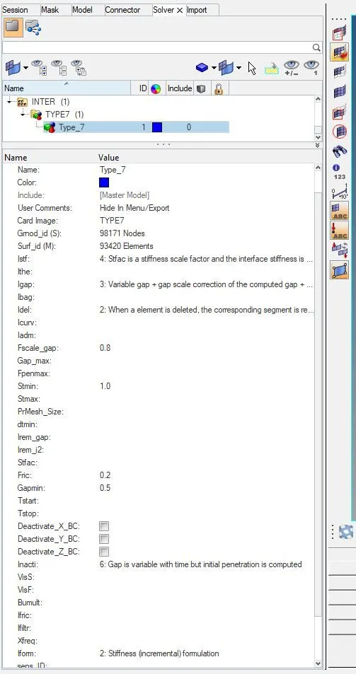
Figure 3: Type 7 interface card.

While defining the type 7 interface card, the preventive measure has been taken to avoid any initial penetration or intersection, if any exist. Yet it is better to check manually if any penetration exists in the model. To check that, there is a tool in Tools → Penetration Check. The complete component was selected to check for any penetration in the whole model. When the tool checked the model, it found no penetration in the model, which was a good sign.

Now, for the crash to occur in the simulation, a rigid wall was required. In the solver deck, right-clicking the mouse and selecting the Create → RWALL → PLANE, a plane rigid wall card gets created, as shown in fig. 4.

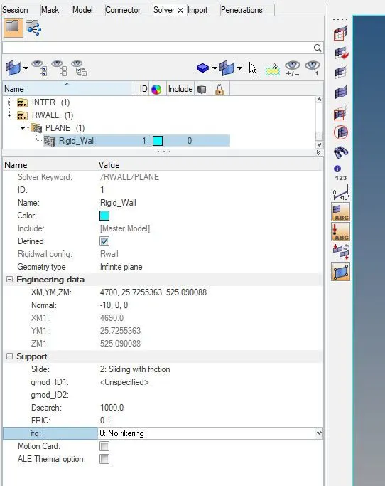
Figure 4: Plane rigid wall card.

The XM, YM, ZM is the co-ordinate of the base node, which was selected from the outer-most area of the bumper. The direction of the normal vector was given towards the vehicle. In the Support → Slide, it was kept to the ‘Slide with friction’, and the FRIC value was given as 0.1. The Dsearch, which is a search distance, is given as 1000. Fig. 5 shows the view of the rigid wall.

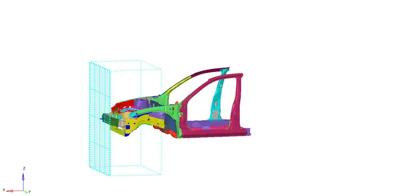
Figure 5: Rigid wall provided for the crash to occur.

It was required to keep the overall mass of the vehicle to 700 kg, however, using Tools → Mass Details → Mass, Cog, and Inertia, it was found that the existing mass of the vehicle was only 188 kg. Also, the COG must be in line with the cross beam of the driver seat, which is not there as required, as can be seen in fig. 6.

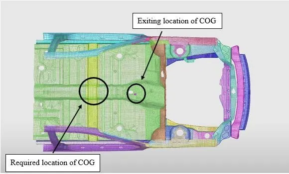
Figure 6: Existing location of COG had to be changed to the required location, by adding mass at the rear.

In the solver tab right-clicking and selecting Create → ADMAS, a mass can be added on the set of nodes. Selecting this tool, a mass was adjusted in the rear as well as front, to bring the cog on the cross beam of the driver seat, and to increase the overall mass of the vehicle to 700 kg.

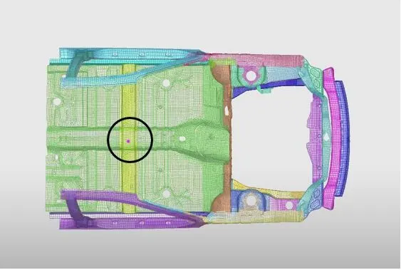
Figure 7: COG was brought to the desired location, by adding some mass at the front and rear.

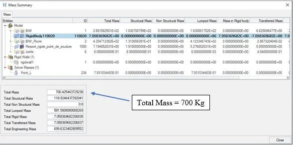
Figure 8: Total mass of the vehicle is increased from 188 kg to 700 kg.

When the model is ready for the simulation environment, boundary conditions are required for the simulation to occur. In this crash project, the initial velocity is one of the boundary conditions. The initial velocity of 35 mph to be applied to the vehicle. Because, the working unit is [Kg mm ms], the initial velocity is 15.6464 mm/ms. Fig. 9 shows the INIVEL card with all values mentioned. To apply the initial velocity, right-clicked in the solver tab, and selected Create → BOUNDARY CONDITIONS → INIVEL. In that INIVEL card, all the components of the vehicle were selected for assigning the initial velocity, and the velocity of 15.6464 was applied in the x-direction, i.e., in the direction of the rigid wall.

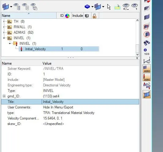
Figure 9: INIVEL card to assign initial velocity.

Now, the time-step was required to be 0.5 to 0.1 microseconds. Thus, in the Cards of Model tab, ENG_DT_NODA is opened. In that card, CST0 formulation is selected to maintain constant time-step. The minimum time-step, Tmin of 0.5 microseconds, or 0.005 ms, Tscale of 0.67 is applied, as shown in fig. 10.

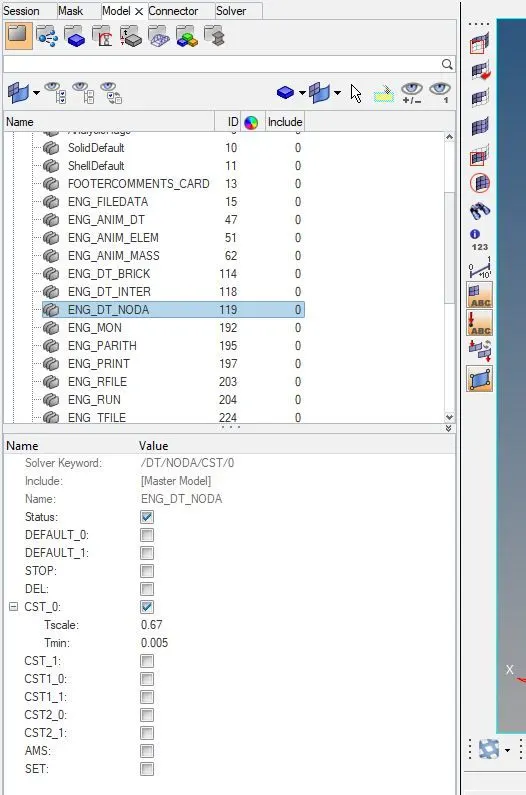
Figure 10: ENG_DT_NODA card with 0.5 microseconds of time-step applied.

The engine run-time was required to be 80 ms. Thus, in the Cards of Model tab, the ENG_RUN card was opened. In that, the Tstop value changed to 80 ms, as shown in fig. 11.

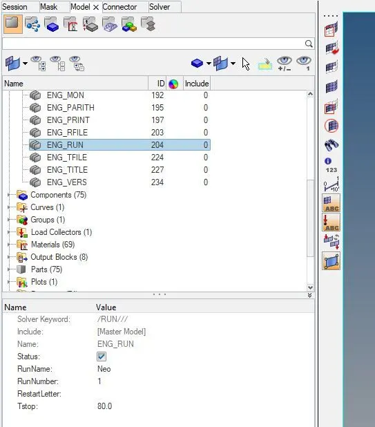
Figure 11: ENG_RUN card with Tstop value of 80 ms.

For getting the desired results like sectional force in rails, axial force on rails, shotgun cross-sectional forces, forces on A-pillar cross-section, etc. a moving frame is required. To create the moving frame, right-clicked in solver tab, and Create → FRAME → MOV was selected. It was a moving frame card, using which a moving frame was created corresponding to the global coordinate., as can be seen in fig. 12.

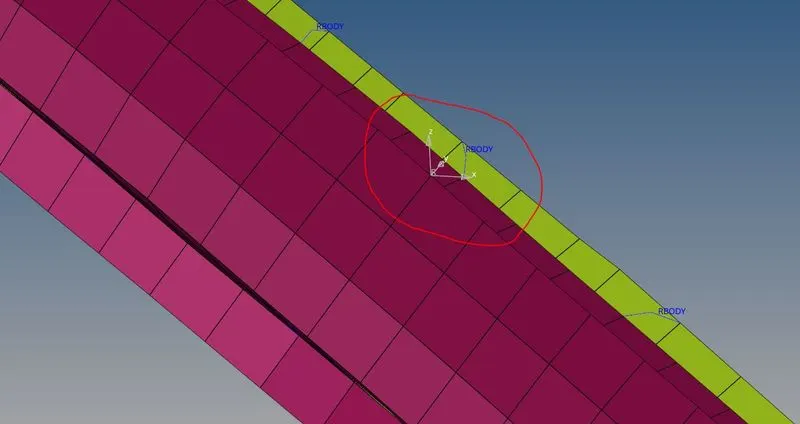
Figure 12: Moving frame on A-pillar.

After introducing the moving frame, further a cross-section is also required around that frame. Thus, right-click in the solver tab, and Create → SECT → SECT was selected. In that card, Frame_ID was the moving frame that was created, grshel_id was the set of elements defining the cross-section. After assigning all the parameters, it appears as shown in fig. 13.

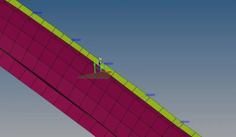
Figure 13: Moving frame and section applied to the A-pillar.

Similarly, this moving frame and section are required on rails, shotgun, A-pillar, and bumper. Moreover, these were required on either side of the vehicle. Thus, in total, 8 frames we required, as can be seen in fig. 14. All of those were created in the same way.

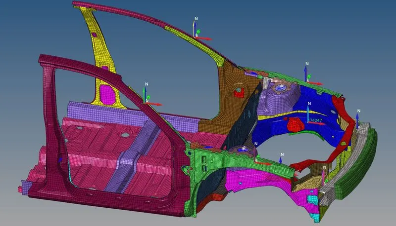
Figure 14: 8 moving frames with all cross-sections defined on 4 parts of the vehicle.

After creating these moving frames and sections, their results have to be requested. Thus, right-click in the Model tab, and Create → Output Block was selected. It requests the time history file. In this card, ENTITY ID is selected as the section that was created earlier. For example, one output block was created for the left A-pillar, given it the name A_Pillar_Left, and ENTITY ID is selected as the section of the left A-pillar. Similarly, such output blocks were created for all the remaining 7 sections.

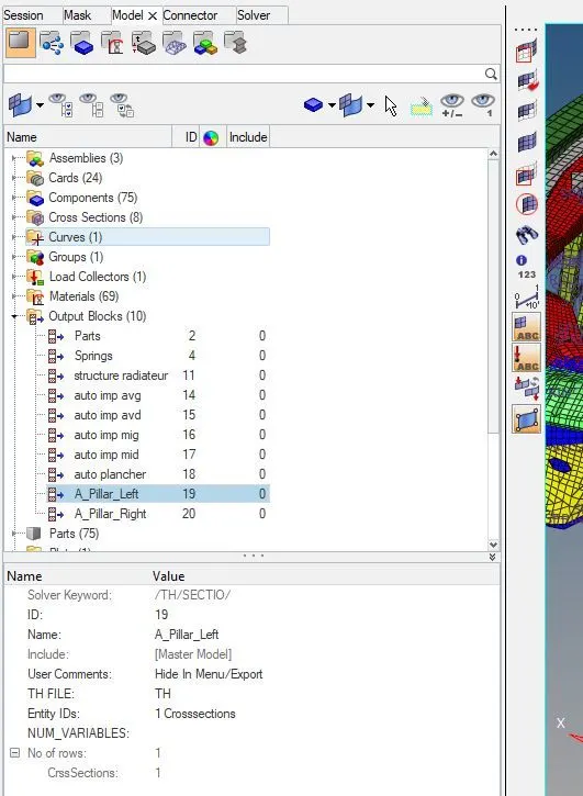
Figure 15: Output block card of left A-pillar.

In the output requests, the vehicle also had to be analyzed for the acceleration at the base of the B-pillar. To get the acceleration curve, an accelerometer is required to put on the pillar. In the solver tab, using Create → ACCEL, an accelerometer card gets created. In that card, node_ID is selected as one of the nodes of the B-pillar, where an acceleration curve is required. Fig. 16 shows the accelerometer put on the base of the B-pillar.

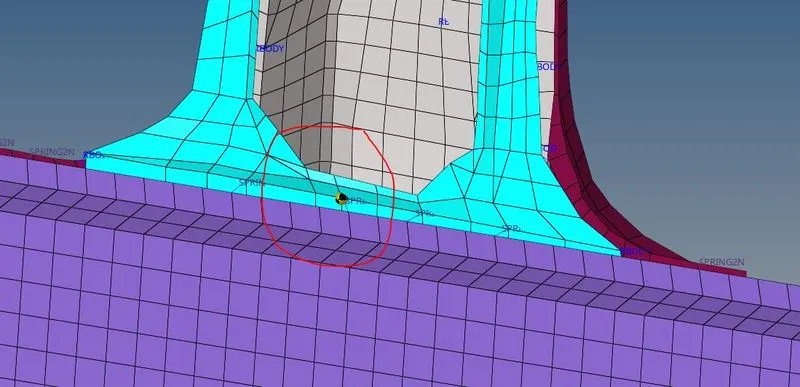
Figure 16: Acceleration put on the base of B-pillar.

After putting the accelerometer, an output request has to be made as done before. Thus right-clicking in the model tab, and using Create → Output Block, an output request was made for the time history of an accelerometer.

One more task of the project was to check the intrusion on two nodes i.e., 66695 and 66244. To do that, a skew was created in line with those nodes by right-clicking in the solver tab and selecting Create → SKEW → MOV. Once created, then, an output block was created in which ENTITY ID is selected as the node on which intrusion has to be analyzed, and Iskew is selected as the corresponding skew in-line with that node.

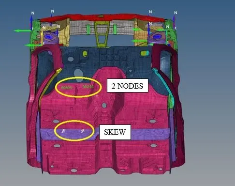
Figure 17: Intrusion created for two nodes by creating two skews.

SOLVER

When the model is ready with all the properties and boundary conditions defined, it is ready for the simulation to run. The model was saved and using Analysis → Radioss, a simulation was run. Four cores of the system were used by giving command -nt 4.

POST-PROCESSING

Output File Check

The run took 363.33 seconds i.e., 6 minutes 3 seconds, to simulate the model, as can be seen in fig. 18.

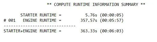
Figure 18: Run takes 363.33 seconds to simulate the model.

However, when the output file was checked, it was found that the energy error was tremendously increased. The increased mass suggests that the elements have gone under huge deformation which led to the addition of nodal mass and eventually increases in kinetic energy and thus increases in the error of total energy.

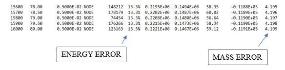
Figure 19: Increased energy error and mass error in the first run.

To reduce this error, the time-step for the model was reduced from 0.005 ms to 0.003 ms and the simulation was run again for the model. Fig. 20 shows the energy and mass error in the second run, and fig. 21 showing the details of computation time.

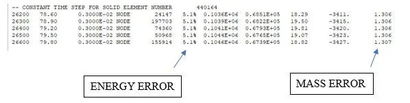
Figure 20: Errors of the second run.

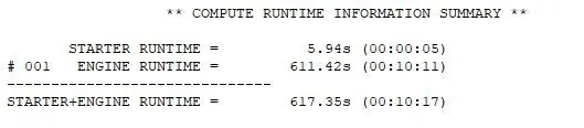
Figure 21: Details of the runtime of the second run.

Comparing fig. 19, and fig. 20, it can be observed that both the mass error and energy error have considerably reduced. The mass error has been reduced by 68.87% and the energy error by 61.65. In the second run, both errors are within the acceptable range. The mass error is less than 1% of the total mass. It is only 0.186%.

But one should also focus on the increased computation time. The run-time earlier took 363.33 seconds to solve the problem, however, in the second run, it took 617.35 seconds. It means the run-time also increased by 69.91%, which is a very huge time for a full-scale model.

Contour Plot

Fig. 22 shows the Von-Mises stresses developed in the vehicle structure, with the maximum value of stress is equal to 342.7 MPa.

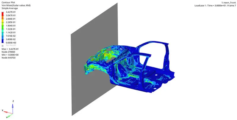
Figure 22: Von Mises stresses developed in the vehicle structure.

Fig. 23 shows the plastic strain developed in the vehicle structure with the maximum value of 0.793.

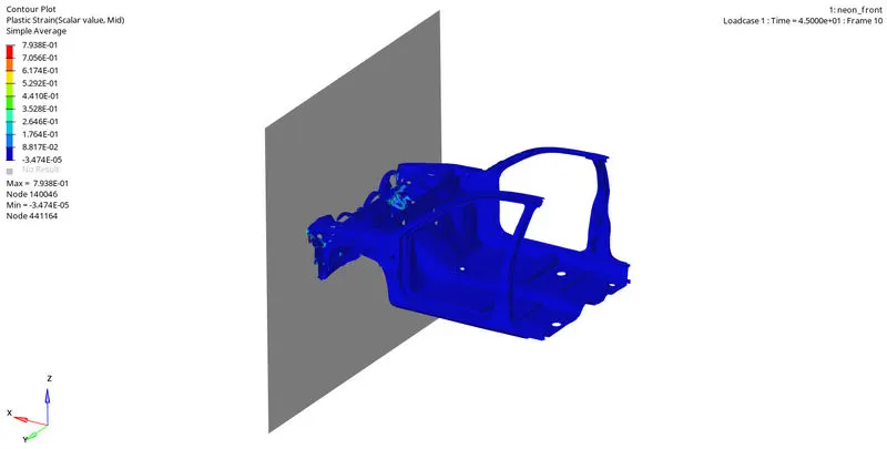
Figure 23: Plastic strain developed in-vehicle structure.

2-D Graphs

Fig. 24 showing the plot of a global variable. It shows that till 13 or 14 ms, the crash has not occurred, and thus the values of kinetic energy (KE), internal energy (IE), and total energy (TE) were constant. Once the crash occurred, the kinetic energy of the vehicle started transferring to internal energy arising due to the deformation of the elements. The contact energy and hourglass energy are negligible; hence they are not part of the concern.

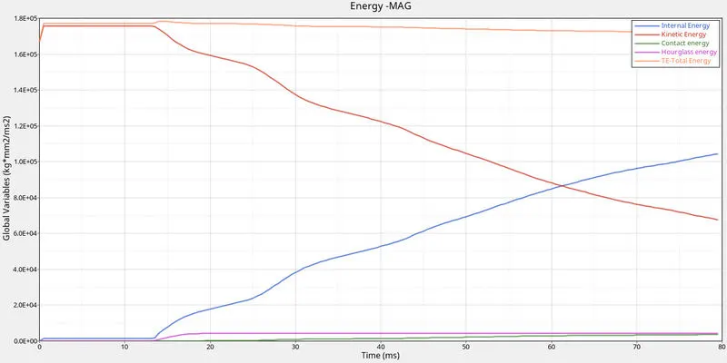
Figure 24: Plot of global variables.

The nature of force distribution in the A-pillar, shotgun, bumper, and rails are shown below.

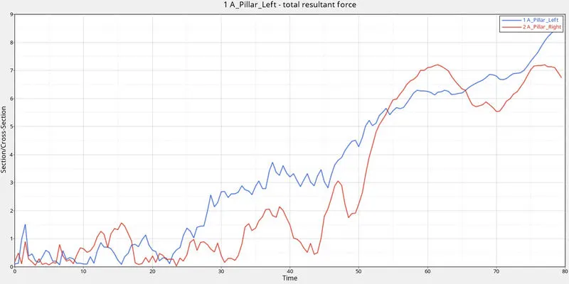
Figure 25: Plot of total resultant force in A-Pillar of both sides.

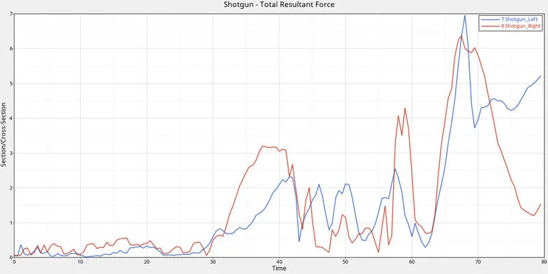
Figure 26: Plot of total resultant force in Shotgun of both sides.

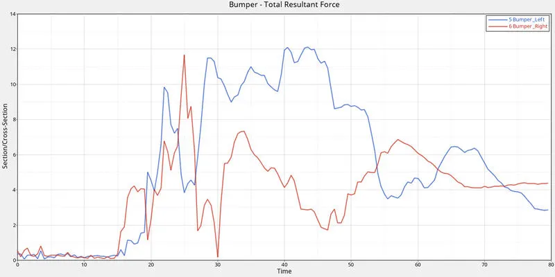
Figure 27: Plot of total resultant force in the bumper on both sides.

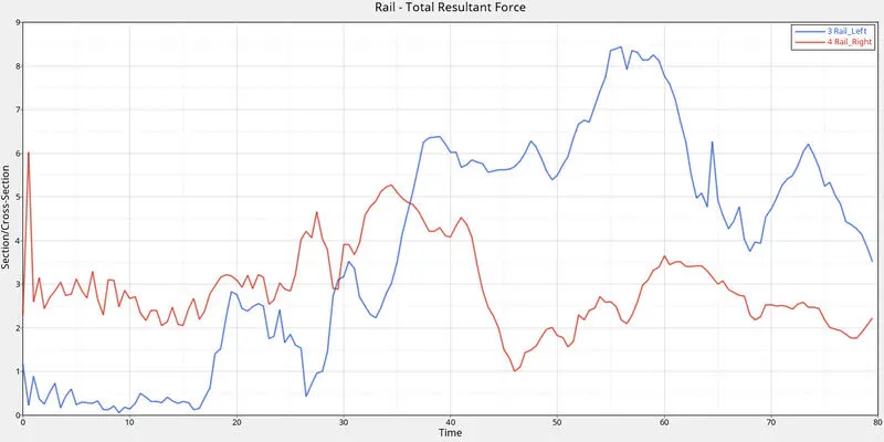
Figure 28: Plot of total resultant force in rails of both sides.

An accelerometer was put on the base of the B-pillar. Its variation w.r.t. time is shown in fig. 29.

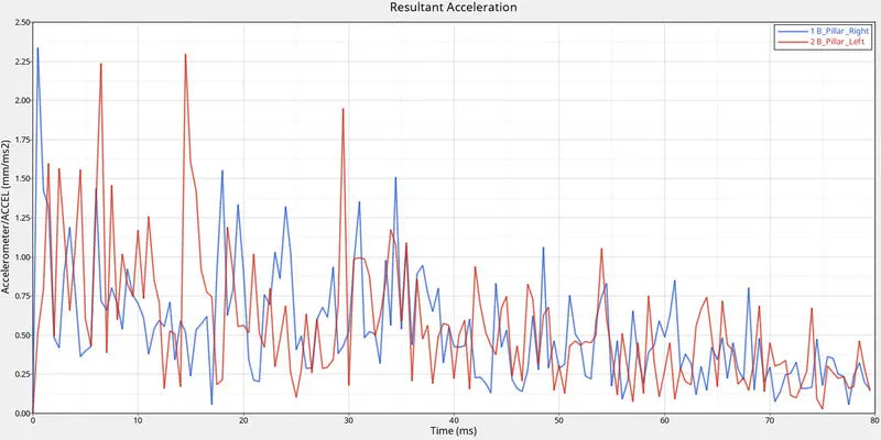
Figure 29. Acceleration at the base of the B-pillar.

The intrusions on dash-wall nodes 66695 and 66244 are shown in fig. 30.

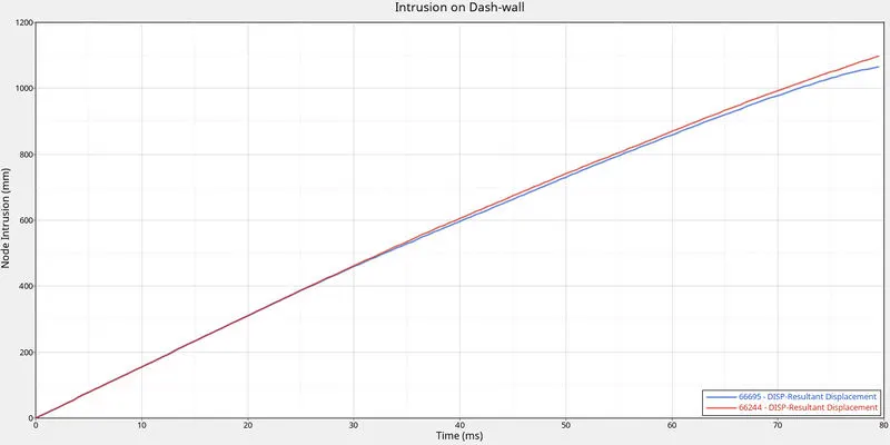
Figure 30. Intrusion in the nodes of dash-wall.

Result and Discussion

The model of vehicle structure was not the full-scale model. There was a limitation of software of 100k nodes. Thus, the length of the model was reduced to 100k nodes. Initially, the mass of the vehicle structure was 188 kg which was required to be 700 kg. Also, the cog was not in line with the cross-beam of the driver seat, which has to be its location. Thus, some mass was added in front as well as rear to make the mass of the vehicle structure 700 kg and bring the COG point in line with the cross beam of the driver seat. Next, the existing interfaces of the vehicle were deleted and made to type 7 interface, which is a general node-to-surface contact with the self-impacting property.

A rigid wall is put ahead of the vehicle for the crash to occur, and an initial velocity of 35 mph or 15.6464 mm/ms is given to it. The nodal minimum time-step of 0.5 microseconds or 0.005 ms with a scale factor of 0.67 is given. And the run-time was set to 80 ms.

The forces were required to check on the cross-section of the A-pillar, shotgun, bumper, and rails. Thus, a moving frame was put on those parts and provided sections. An accelerometer was put on the base of the B-pillar. Intrusion had to check on the nodes of the dash wall. Thus, the moving skew was made to check the intrusion. After creating all the required results, a TH file or time-history file was requested by creating an output block for all.

When the simulation was run for the first time, it took 6 minutes and 3 seconds to solve. When the output file was analyzed, it showed that the result had a 13.3 % of error with 4.199 kg of mass error, which was not very good enough to accept. The mass addition on nodes shows that a huge amount of deformation has been occurred, which led to the increase in the density and ultimately the reduction in time-step. To get the acceptable results, the time-step was reduced to 0.3 microseconds, and the simulation was run one more time. This time the energy error was reduced to 5.1% with the mass error of only 1.307 kg which is 0.186%. Now, it was quite a good and acceptable result. However, due to the reduction in time-step, the computation time was increased by 69.91% which is a very huge time to consider.

In the contour plot of Von Mises, it can be observed that a huge of stress developing on the front of the vehicle is spread across the vehicle structure, and thus less stress or almost no stress is developing on the seat’s crossbeam. It is a good sign that driver’s seat cross beam is safe from incoming stresses.

The plot of global variables shows that as soon as the crash occurred, all of the kinetic energy of the vehicle started transferring to internal energy which arose due to the huge deformation in the frontal region of the vehicle structure. From fig. 25, fig. 26, fig. 27, and fig. 28 it can be observed that initially, the force came on the right rail, at first. Because the right rail has taken initial force, there is less force transfer in the right A-pillar, right bumper, and right shotgun compared to their corresponding other sides. After rails, the A-pillar has continuously taken incoming loads. The bumper has taken the load until 60 ms. After that, it might have crumbled completely.

The acceleration in B-pillar also shows that the first sudden move occurred on the right side. The acceleration initially was huge, when the crash occurred. Once the force started distributing, the acceleration started reducing. The intrusions on nodes of the dash wall show that there was a displacement of 1100 mm have occurred.

CONCLUSION

The crashworthiness of this vehicle suggests that very little or almost no stress is transferring to the occupant. Many of its load is taken by rail, shotgun, A-pillar, and most important the bumper. However, the intrusion of 1100 mm also suggests that some more improvement is also required to increase the crashworthiness. This model of vehicle is not the full-scale model, therefore, the collected information is also not fully-scaled one. However, it gives a general understanding of how forces get transfers to the structure, and how the industry works to keep the occupant safe from any crash.