Assignment 6-Frontal Crash Simulation Challenge

OBJECTIVE :

• To perform frontal crash analysis of a vehicle against a rigid wall in Hypermesh.
• To simulate the crash behavior of the vehicle in HyperView and discuss the results.
• To plot the sectional and axial forces at different locations and discuss the results.
• To obtain intrusion results at dash wall and plot them in HyperGraph.
• To obtain acceleration and plot acceleration curve at B-Pillar.

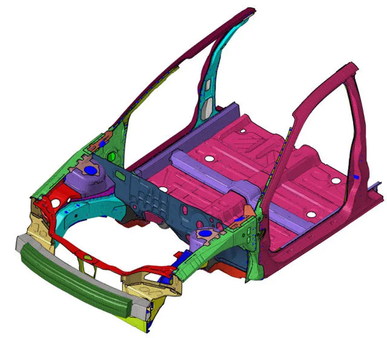
MODEL:

PROCEDURE:

1.Import the 0000.rad starter file into the hypermesh GUI.

2.Check for the units system in the BEGIN CARD and follow as mentioned in the question.(kg mm ms)

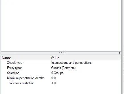
3.Check for penetrations in the model by Tools-penetration check

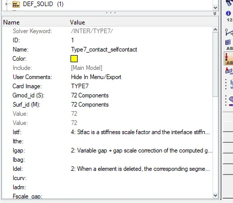
4.For this model, we will create Type 7 interface for all the components of the model as it is self-impacting or the nodes and elements of the model will have a contact between them. We will go to Solver browser and we will delete all the existing interfaces. Then we will right click and navigate to Create > INTER > TYPE 7. Under Type 7 interface card, we will select all the components for slave nodes and master surface in Grnod_id(S) and Surf_id(M) respectively. Then we will define all the recommended parameters for Type 7 interface i.e. Istf = 4, Igap = 2, Idel = 2, Fscale_gap = 0.8, Stmin = 1 kN, Fric = 0.2, Gapmin = 0.5, Iform = 2. Here we will define Inacti as 0 which is default because there are no penetrations in the model.

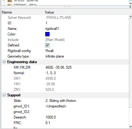
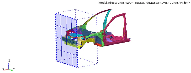
5. To create a plane rigid wall at the front side of the car, we will need the outermost node at the bumper of the car. So we will create the outermost node on the element edge using temp nodes option. Then we will right click in solver browser and navigate to Create > RWALL > PLANE. For the location of rigid wall, we will click on the node which we created and then give a gap of 10 mm in X-axis as the wall must not be connected to the model. The normal of the wall will be in negative X-axis i.e. -1,0,0. Then we will specify the other parameters as follows.

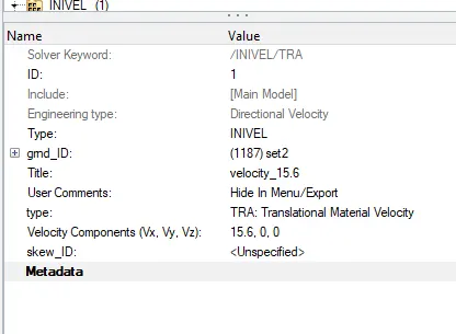
6. To create initial velocity, we will right click on Solver browser and then navigate to Create > BOUNDARY CONDITIONS > INIVEL. Under INIVEL card, we will select all the components as the Entity for grnd_ID. We will give the initial velocity of 35 mph or 15.6464 mm/ms in X-axis and as the velocity should be translational velocity, we will select TRA option in type.

7.

Cross Section –

The results which we want on required cross sectional parts will be calculated based on a frame of reference. So before creating cross section, we will create moving frames on a particular node of that section. Now as we have to create the moving frames which are also called as local axis, we have to perfectly align our local axis to the global axis. So for this, we will extract the node location or coordinates of a particular node on the section in nodes panel. 

Now we can create moving frame using these nodes. In Solver browser, we will right click and navigate to Create > FRAME > MOV. So here, we will create frame by node reference and select the nodes for x-axis and xy plane and then click on create.

Thus a moving frame will be created. Now we will create cross section for this frame. To create a cross section, we will right click on the Solver browser and navigate to Create > SECT > SECT. In section panel, we will specify the Frame_ID as the moving frame which we created.We will right click and create grshel_id, then we will select the elements where we want the cross sectional results.

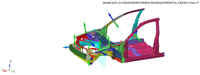
Similarly, we will create the cross sections at required parts namely A-pillar, Shotgun or Fender, Bracket and Rail. These cross sections will be created at both the sides i.e. left side and right side of the vehicle as shown below.

8.

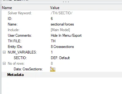
After creating the cross sections, we will request the results in TH or time history. For this we will go to Output Blocks under Model browser. Then we will right click and create a new output block. Under Entity IDs option, we will select the cross section which we created and thus we will be able to plot graphs of the cross sectional forces in HyperGraph.

9. Accelerometer –

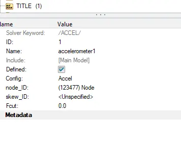
We have to measure acceleration of B-pillar during the crash. So we will create accelerometers on both the B-pillars. To create accelerometer, we will right click in the Solver browser and navigate to Create > ACCEL. Then in node_ID, select the node on the B-pillar where we want acceleration result and specify F_cut value as 1.65.

10.

Intrusion –

Here, we need to find the intrusions on the dash wall at node 66695 and 66244 respectively. So to find the results at the specified nodes, we need to have a frame of reference. Thus we will create moving frames at Seat reinforcement part which is shown below.

11.

Mass Addition and Balancing (Required mass - 700 kg) –

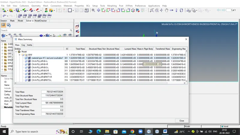
At first, we will check mass and CG of the vehicle by Tools-mass and cog check

In general, the CG of the vehicle is somewhere just behind the driver’s seat. So in order to get the required CG location, we will do mass balancing by adding some on the panel where the passenger seats are located. We also have to get the mass of the vehicle to 700 kg. So in Hypermesh, under solver browser, we will right click and navigate to Create > ADMAS. In ADMAS panel, we will specify the required mass to selected nodes and for Mass type, we will select Mass/node option.

In this way, we will create Rear_Mass and Front_Mass and balance them to get 700 kg and Cg at required position. Since this model is not the complete vehicle model, the point of CG which will be obtained won’t represent real life scenario. Thus we will not concentrate much on the Z-axis of the CG point and we will get CG below the floor panel as shown below.

12.

Time Step and Run time –

To check these parameters in Hypermesh, we will navigate to Cards under Model browser. To check the run time, we will open ENG_RUN card where we will see that the model already have the run time in Tstop as 80 ms. For the time step, we will open ENG_DT_NODA card and we will change the Tmin value to 0.5 microseconds or 0.0005 ms.

13. 

Model Checker –

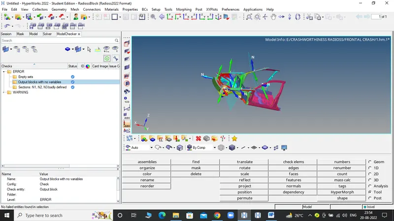
To check the quality of the model in Hypermesh, in Menu Bar we will navigate to Tools > Model Checker > RadiossBlock. This will open a new Model Checker browser

In this browser, we will click on Run checks command which is at the top right side in the above figure, indicated in red box. After running the checks, we will click on Auto correct command which is in blue box, through which the software will automatically perform the possible corrections and give a green tick in status bar.

14.

Now we can proceed to run the simulation. So we will navigate to Radioss in Analysis page. Here we will save the model to a specified path and in options, we will type –nt 4 and then click on Radioss option to run the analysis.

SIMULATION AND RESULTS :

First, we will check Energy error and Mass error. So we will open the engine .out file of the model and check the last column for Energy and Mass error as shown below.

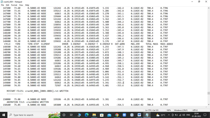
The  Energy error which is -0.2% and  Mass error which is very negligible. This shows that the energy error and mass error are within acceptable range.

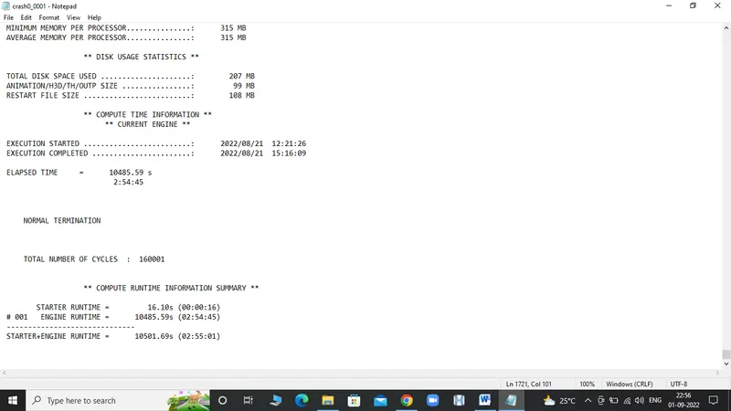
The total number of cycles used is 160001 and the total runtime of the simulation is 10501.69 s.

To view the simulation results, we will switch to Hyperview. In Hyperview, we will load .h3d file from specified path and we will play the simulation.

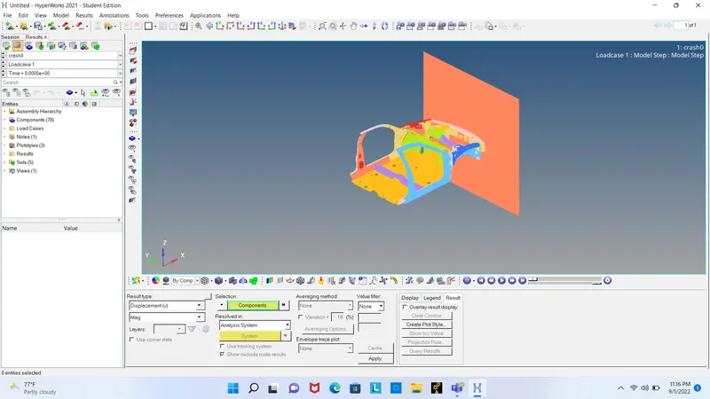
In the above crash simulation of the vehicle, we can see the vehicle body is impacting on the rigid wall. After the impact, the frame of the vehicle deforms and the vehicle has a pitching movement about its CG point. As this model is a reduced model and not a complete model, the deformation is unrealistic.

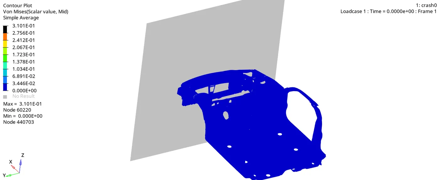
From the Von Mises stress plot, we can say that the stress distribution is quite good in the vehicle after the crash. There are very few areas where we can see stress concentration. Generally the stress is more in bumper region as it is the first point of impact.

PLOTS AND ENERGIES:

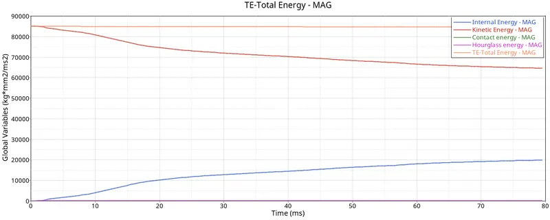
From the above plot, we can see that there is high amount of Kinetic energy at the start of the simulation but as the simulation progresses, the kinetic energy in the vehicle decreases and the internal energy increases in the same proportion. Thus the total energy in the system is almost constant at 85000 J and due to some energy loss which we can see in energy error, there is some decrease in total energy. We can also see some amount of contact energy in the model as we have defined the value of friction in Type 7 interface due to which contact energy is generated.

Cross Sectional Forces –

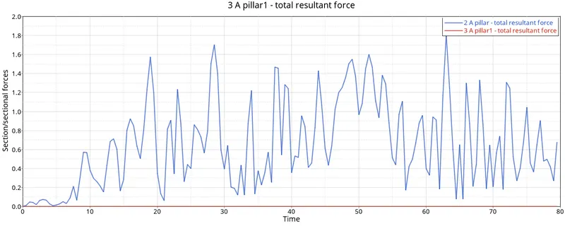
A-Pillar 

Shotgun –

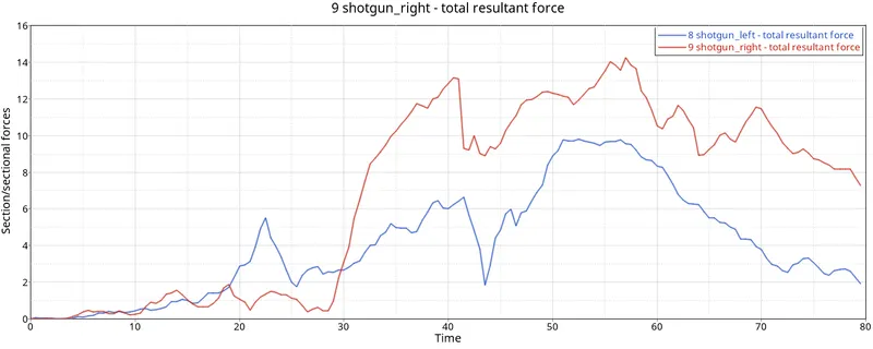
From the above plot, we can see that initially the resultant forces experienced on the left side Shotgun was higher but as the simulation progresses, the forces at right side Shotgun is much more than that experienced on the right side Shotgun.

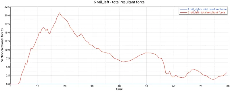
RAIL:

Accelerometer –

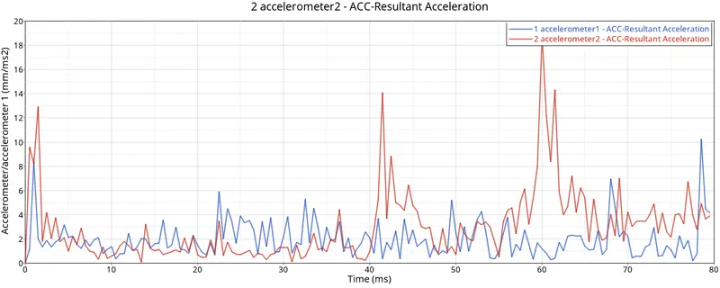
Initially, the acceleration of the both b pillars were almost similar but as the simulation progresses, the acceleration of the left B-pillar is more than right B-pillar. The maximum acceleration of right B-pillar is 18 m/s² whereas the maximum acceleration of left B-pillar is 10 m/s².

Intrusions

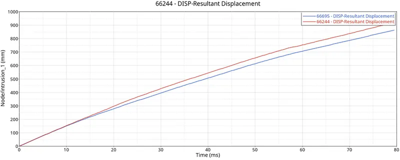
The resultant displacement at node 66244 is 900 mm and the distance between the node 66244 and node of its respective skew is 793.73 mm. Thus the intrusion at node with ID 66244 is 900 – 793.73 = 106.27 mm. Similarly the distance between the node ID 66695 and node of its respective skew is 767.62 mm and the resulting intrusion is 900 – 767.62 = 132.38 mm.

CONCLUSION :

The vehicle model is impacted on a rigid wall to study the frontal crash scenario of the vehicle. As the model is reduced to limited parts, we got unrealistic deformations and results. Thus the center of gravity of the vehicle along with vehicle mass is very important and it mainly decides the behavior of the vehicle under crash.