Frontal Crash Analysis of Dodge Neon

OBJECTIVE:

To perform a Frontal Crash Analysis on the BIW structure of Dodge Neon and study how the impact forces are distributed throughout the chassis to keep the occupants safe.

PRE-REQUISITES:

i) A crash simulation is a virtual recreation of a destructive crash test of a car using a computer simulation in order to examine the level of safety of the car and its occupants.

ii) Crash simulations are used by automakers during Computer-Aided Engineering (CAE) analysis for crashworthiness.

iii) During a crash simulation, the kinetic energy that a vehicle has before the impact is transformed into deformation energy, mostly by plastic deformation of the car body material at the end of the impact.

iv) ­The dummy's job is to simulate a human being during a crash while collecting data that would not be possible to collect from a human occupant.

v) The dummies contain three types of instrumentation namely Accelerometer, Load sensors and Motion sensors.

vi) In this case, we will be conducting a frontal crash analysis of Dodge Neon.

vii) The car is set at a velocity of 35mph and is made to crash into a solid concrete barrier in a controlled environment.

viii) Before the crash-test dummies are placed in the vehicle, researchers apply paint to them.

ix) Different colors of paint are applied to the parts of the dummies' bodies most likely to hit during a crash.

x) Researchers analyze the different forces acting on the dummy and determine the safety rating of a car.

PROCEDURE:

a) Initial Setup:

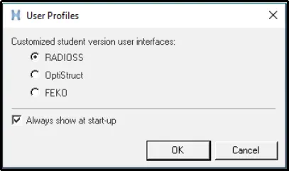
i) Select Radioss from the user interface menu.

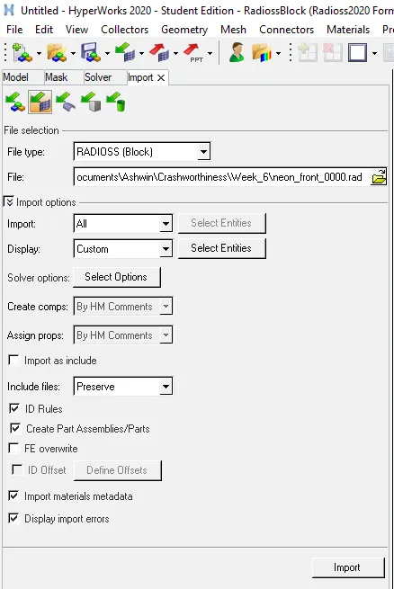
ii) First, we need to import the model into Hypermesh.

iii) To do so, click on Import -> Import Solver Deck -> Choose the starter file -> Import.

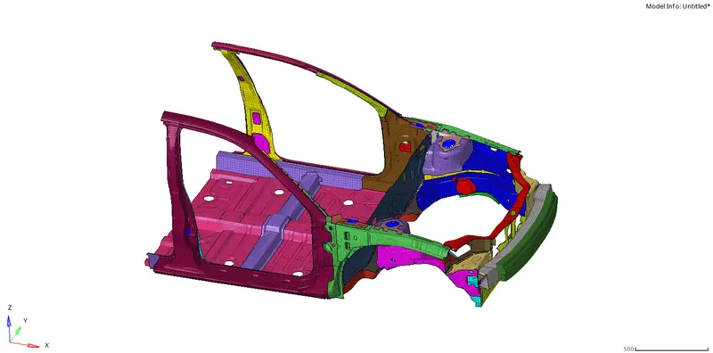
iv) After importing the following model is obtained:

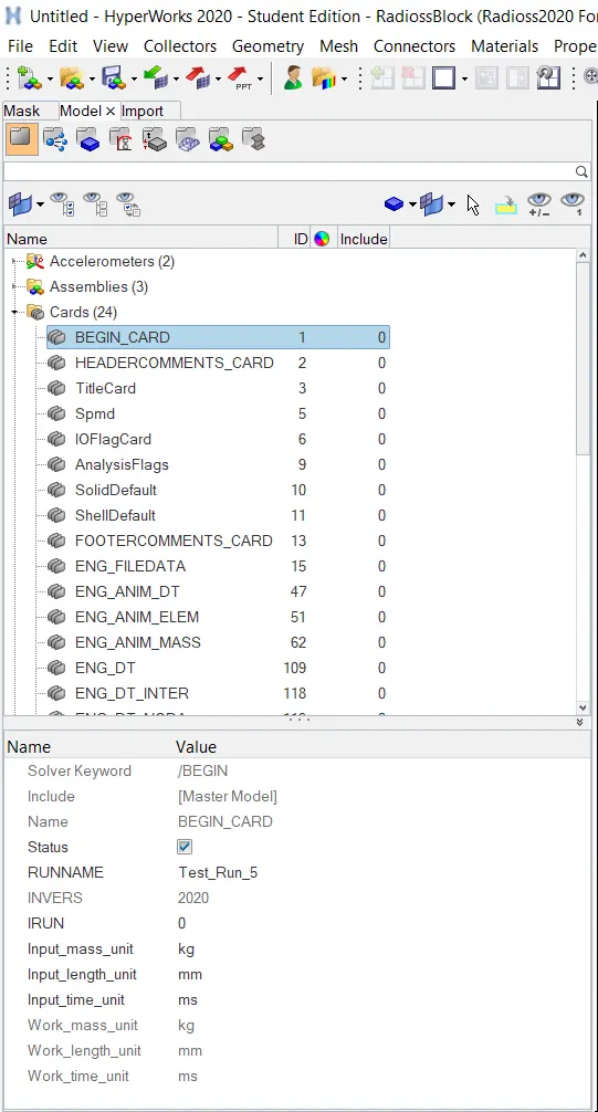
v) Check the unit system by clicking on Model -> Cards -> BEGIN CARDS

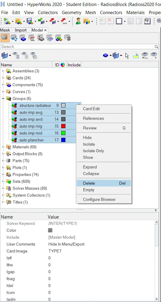
vi) Delete any existing interfaces by clicking on Model -> Right -click on Groups -> Delete.

b) Checking for Penetrations:

i) Due to various reasons like clearing elements for warpage, there is a chance of initial penetration between elements that need to be cleared.

ii) This can be done in Hypermesh as well as HyperCrash.

iii) To do the same in HyperCrash, click on Contact Interface -> Check penetrations for selected objects -> Select All the components

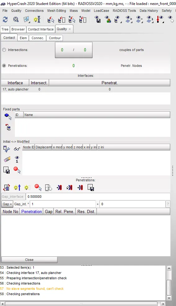
iv) From the above image we can see that there are no initial penetrations.

c) Adding Mass:

i) Ideally the Center of Gravity(COG) of the car should be as low as possible in the middle of the car.

ii) This aids in better handling and ride control.

iii) Since the student version of Hypermesh supports only one lakh nodes, only the front section of the car is meshed.

iv) Therefore the weight of the given model is just 187 kgs.

v) But, to get accurate simulations we need to add the total mass of the vehicle manually (ie. 700-187=513kg).

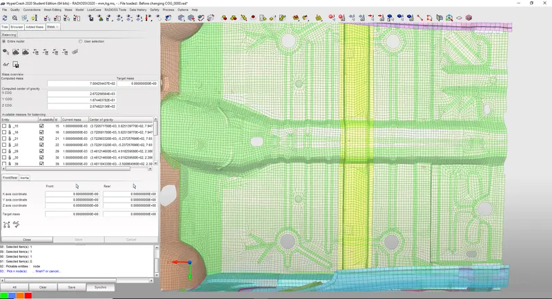
vi) We have to add the mass in such a way that the COG of the car is on the middle crossbeam.

vii) This can be done in Hypermesh as well as HyperCrash.

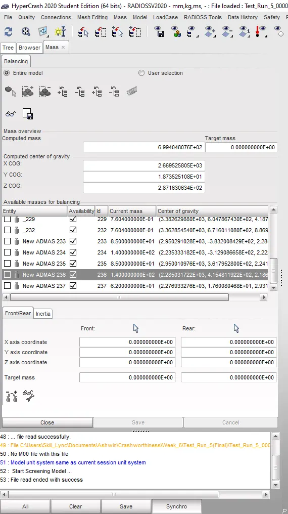
viii) To do the same in HyperCrash, click on Load Case -> Added Mass -> Create new -> Type 1 mass -> Select the nodes -> Add mass -> OK.

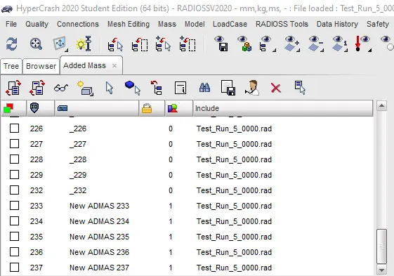
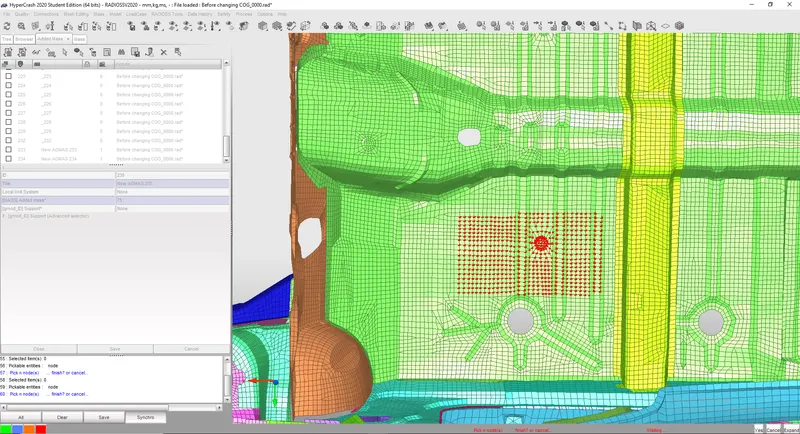
ix) After adding the mass we can see that the total mass of the vehicle is approximately 700 kg.

x) We can see that the COG has been shifted to the middle crossbeam:

xi) Now we can export the file as a .rad file to continue the rest of the analysis in Hypermesh.

xii) To do so, click on File -> Export -> Radioss -> Select folder -> OK.

d) Creation of Rigid Wall:

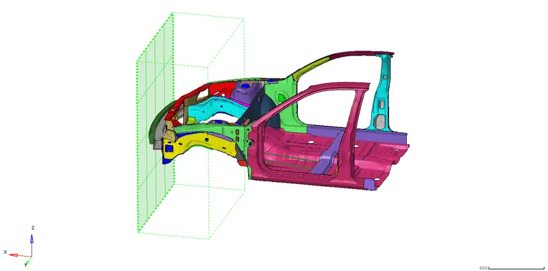
i) Here the rigid wall represents a wall with very high stiffness to replicate a barrier in crash tests.

ii) To create a Rigid Wall in Hypermesh, we must first decide a point at which the wall must be created.

iii) To do so, create a temp node on the middle of the bumper.

iv) Now we need to translate this node by clicking on Tools -> translate -> Node -> Duplicate -> Magnitude =20 -> Direction along X-Axis -> OK.

[Note: If the distance is kept any higher then the computational time of the simulation will increase and also we do not need any results until the car hits the rigid wall]

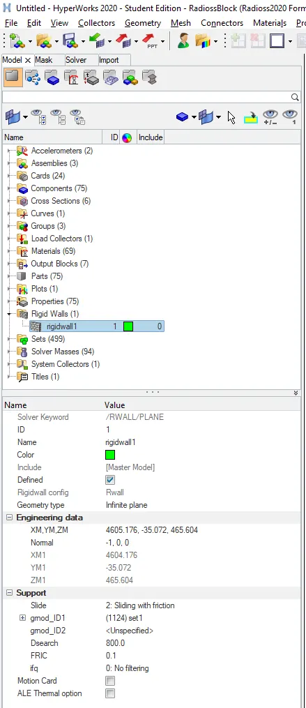
v) To create a rigid wall, click on Solver -> Create -> RWALL -> Plane -> Select the translated node -> Normal= (-1,0,0) -> Slide =2 -> grnod_ID1 = Select all the components of the car as slave -> Dsearch=800 -> Fric = 0.1 -> OK.

e) Creating Interfaces:

i) Since the car will come into contact with itself and other components during a crash, we need to define appropriate interfaces between them.

ii) In this case we will be defining Type 7 contacts.

iii) The recommended properties for Type 7 contact is shown below:

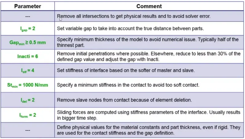
[Note: Stmin=1 for this case ]

iv) First we have to define an interface between the bumper and the headlight bracket on both sides.

v) To do so, click on Model -> Groups -> Create -> Card Image -> Type 7 -> grnod_ID(S)= Select nodes on the bumper -> grnod_ID(M)= Select the headlight bracket as a component -> Select the recommended properties.

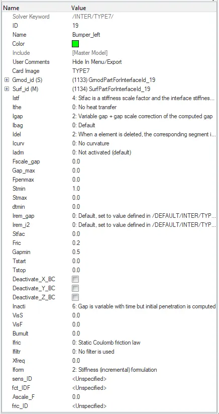
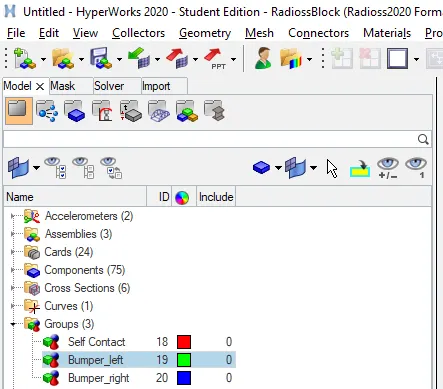
v) Create interfaces for the left and right sides of the bumper using the same procedure.

vi) Also create a self contact with the master and slave being the entire car itself.

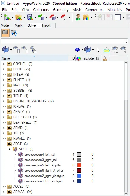
f) Section Forces:

i) The axial forces computed on the section of a component is defined as section force.

ii) To create a section, we need to create a frame first.

iii) To do so, click on Solver -> Create -> Frame -> MOV -> Select the nodes.

iv) To create a section, click on Solver -> Create -> Section -> Select the same nodes as above for N1,N2 and N3 -> deltaT=0.1 -> alpha =0.67

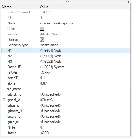
v) Create a section for Left and right Rails, Left and Right Shotguns and left and Right A-Pillars using the same procedure.

g) Timestep and Run Time:

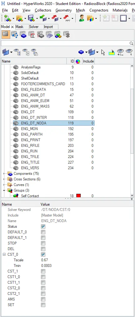
i) To provide time step for the simulation, click on Model -> Cards -> ENG_DT_NODA -> Tscale=0.67 -> Tmin =0.0003.

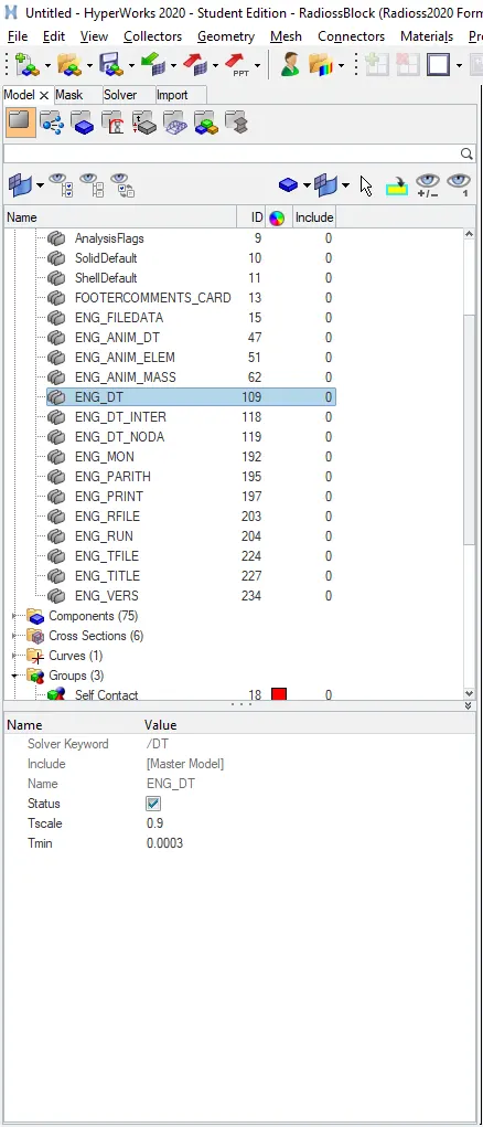
ii) Click on Model -> Cards -> ENG_DT -> Tscale=0.9 -> Tmin =0.0003.

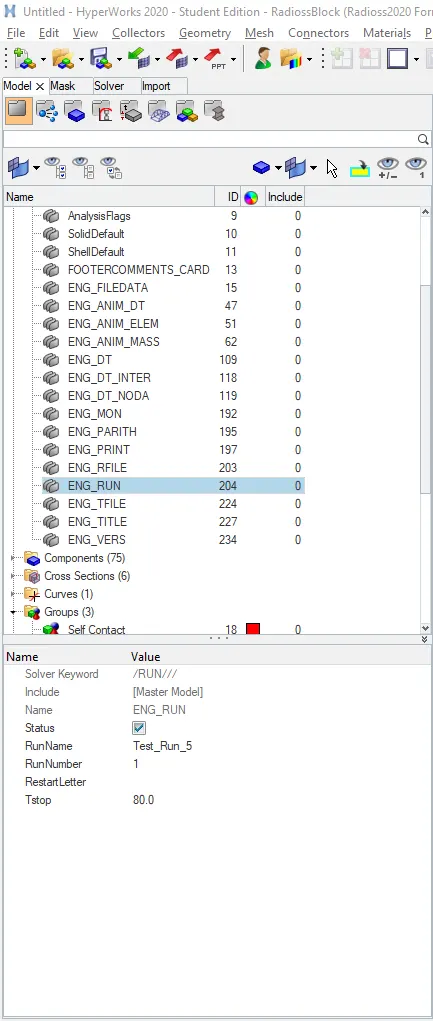
iii) To provide run time for the simulation, click on Model -> Cards -> ENG_RUN -> Tstop= 80.

h) Spring:

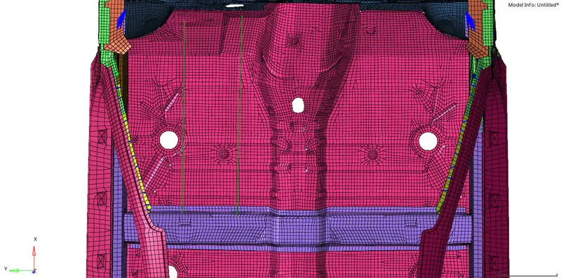
i) To understand occupant safety better, we have to measure any intrusion on the dash wall.

ii) To measure the same we can create springs and measure their change in length during a crash.

iii) To do so, click on 1-D -> Springs -> Spring2 -> Select the two nodes.

iv) We also need to create a spring property.

v) To do so, click on Model ->Property-> Create -> Card Image -> P4_Spring.

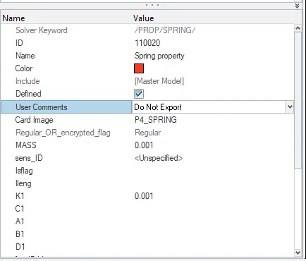
vi) After creating the property assign it to the springs created.

i) Accelerometer:

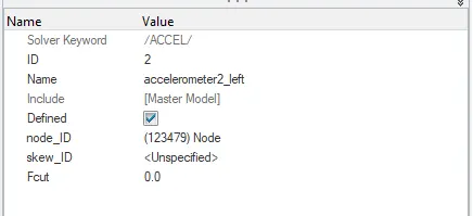
i) We need to measure the acceleration the occupant will undergo during a crash.

ii) To measure the same we have to mount accelerometers on the B-Pillars.

iii) To do so, click on Solver -> Create -> ACCEL -> Select a node on the B-Pillar.

j) Initial Velocity:

i) To simulate a crash, we have to provide initial velocity to the entire car.

ii) As per industry standards, the speed of a car during a crash test is 35 mph.

iii) But the units used in our simulation is mm/ms and thereby convert it.

iv) After conversion the speed needed to be given to the system is 15.64 mm/ms.

v) To provide this value, click on Solver -> Create -> Boundary Condition -> INIVEL -> grnd_ID=Select all the components -> Velocity Components=(15.64,0,0).

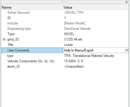
[Note: Velocity is given only to X component as the car is moving in X-Axis]

k) Output Requests:

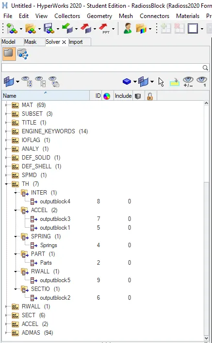
i) After defining all the forces, we need to call them in the output block to view the results.

ii) We have to create output blocks in Solver -> TH for interface force, section forces, accelerometer and spring elongation.

l) Check Connectivity:

i) In order to get proper simulation, we need to make sure there are no free parts in the model.

ii) To check for connectivity, click on Tools-> Find Connectivity -> Select all the components -> Check.

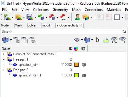
iii) If any free parts are detected we must provide connectivity to them.

m) Model Checker:

i) Before running the simulation, we must check the model for any incompatible kinematic problems or other errors.

ii) To do so, click on Tools -> Model Checker -> RadiossBlock -> Run Checks.

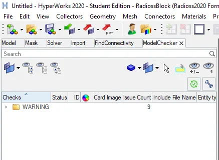
[Note: Model can have warnings but cannot have errors]

iii) Delete any unused or empty components.

n) Running the simulation:

i) To run the simulation, click on Analysis -> Radioss -> Select the file location and name -> Check 'include connectors' box -> Options = '-nt 4' -> Radioss.

[Note: When '-nt 4' is given in the options bar, the simulation will utilize 4 cores of the CPU thereby decreasing simulation time]

RESULTS:

a) Simulation:

i) To view the simulation, switch the menu to HyperView.

ii) Choose the required '.h3d' file from the simulation folder.

iii) The following simulation is obtained:

S.L No	View	Animation
1.	Isometric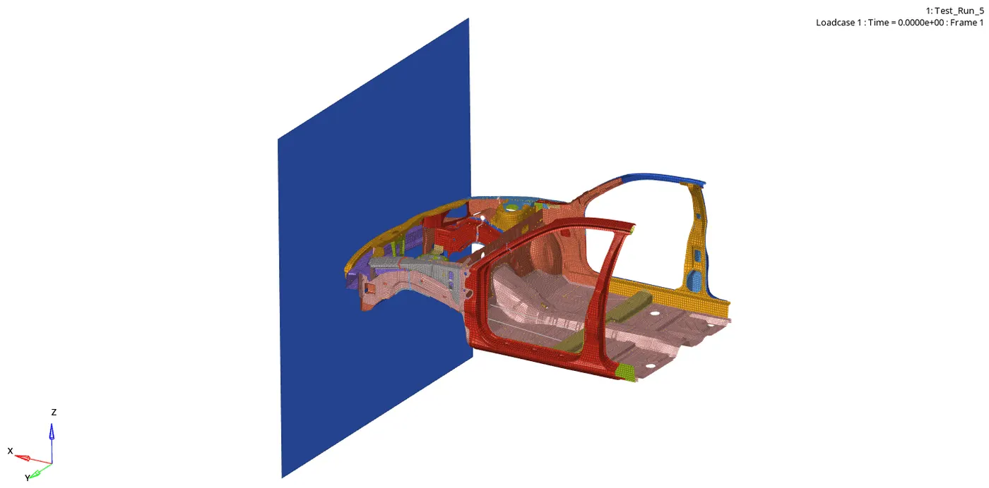
2.	Side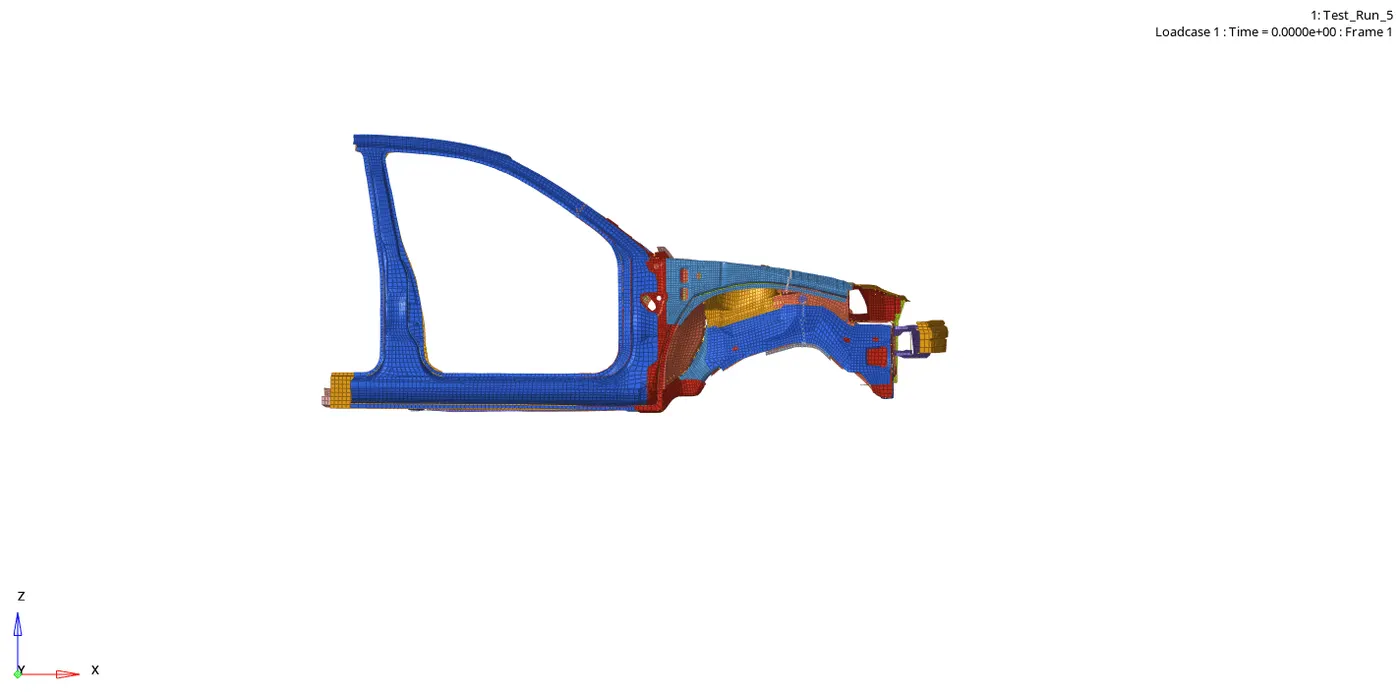
3.	Top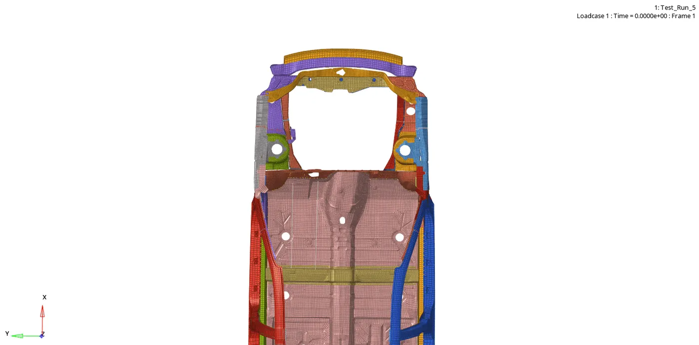

iii) To monitor the displacement in the simulation, click on Contour -> Result type=Displacement(v) -> Apply.

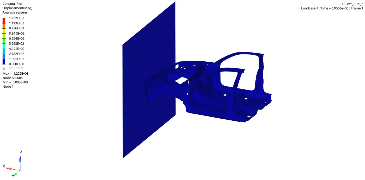
[Note: The maximum displacement obtained was 1252mm]

iv) To monitor the von mises stress in the simulation, click on Contour -> Result type=Von Mises(s) -> Averaging Method= Simple -> Apply.

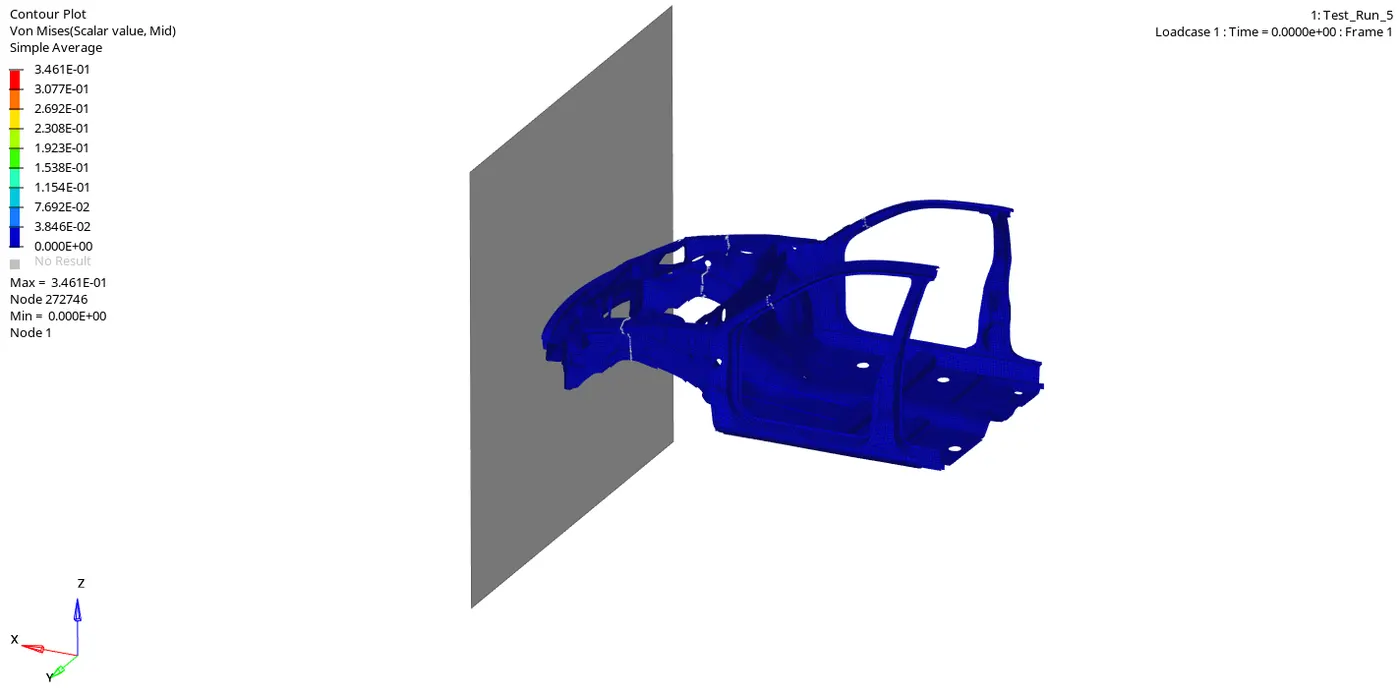
[Note: The maximum Von Mises stress obtained was 0.34GPA]

b) Energy and Mass Error:

i) Energy and Mass error can be found in the '0001.out' file.

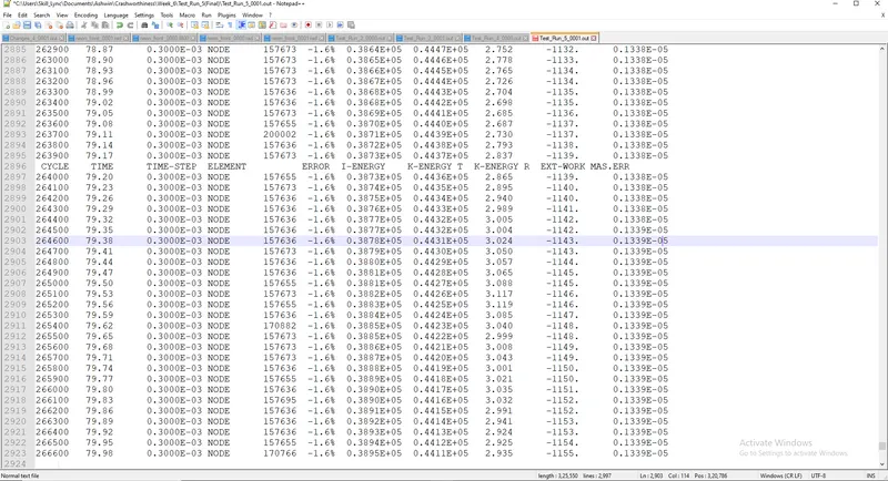
ii) From the above image we can see that the Energy error is -1.6% and Mass error is 0.1339E-05 which are acceptable values.

[Note: The Energy error must not cross 5% and mass added must be very less]

c) Energy Graphs:

i) To plot the graphs we have to switch to HyperGraph 2D.

ii) Select the required T01 file from the simulation folder.

iii) The below-shown graph represents the Internal Energy and Kinetic Energy in the system:

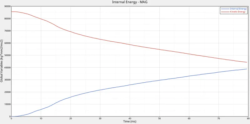
iv) The high kinetic energy in the beginning is due to the motion of the car itself.

v) This slowly decreases due to the impact of the car on the rigid wall.

vi) This kinetic energy is now getting converted to strain energy due to the deformation of the car.

vii) Here, strain energy is nothing but Internal Energy.

viii) Therefore we can conclude that the kinetic energy of the car is getting converted to internal energy.

ix) The below-shown graph represents the contact energy and hourglass energy in the system:

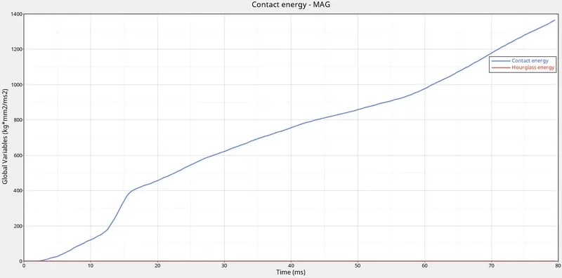
x) Hourglass energy which is an artificial energy is 0.

xi) Contact energy which is the friction energy caused due to two bodies coming in contact, is significantly lesser than Kinetic or Internal energy.

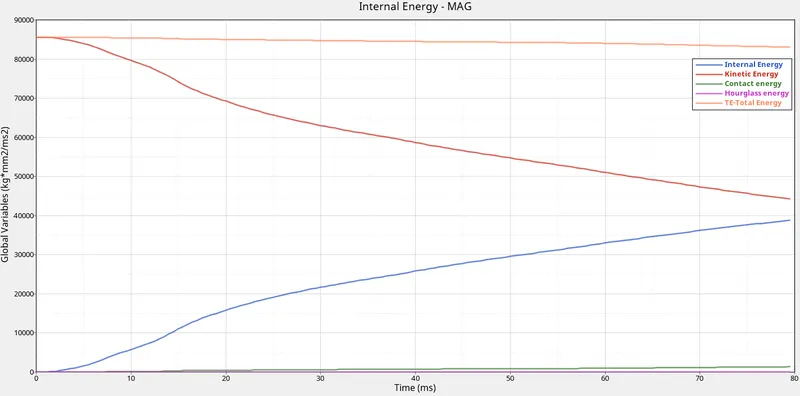
xii) The below-shown graph represents all the energies in the system:

d) Energy Transmission Graphs:

1. Bumper Interface Force:

i) The below-shown graph represents the section force obtained on the bumper:

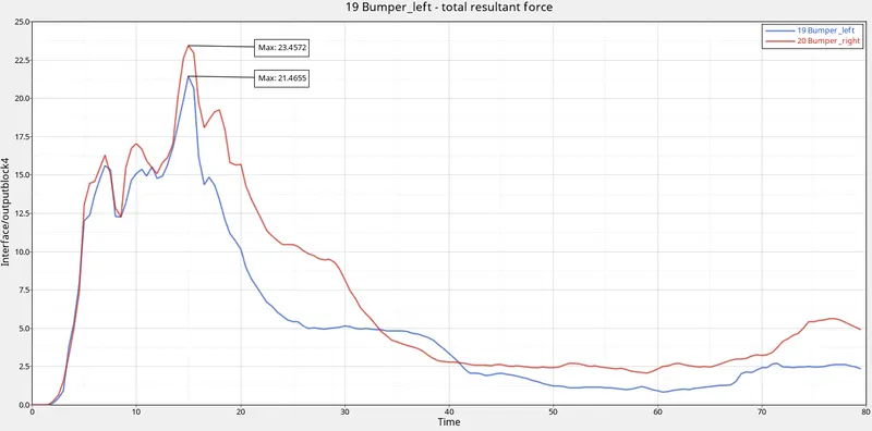
ii) Since the Bumper is the first contact with the wall it absorbs most of the forces.

iii) The maximum force the bumper can take is reached between 10-15ms and then deforms gradually.

iv) The right rail can take more force (23.45KN) than the left rail (21.46KN) due to the unevenness of the bracket on both sides.

2. Rail Section Force:

i) The below-shown graph represents the section force obtained on the rail:

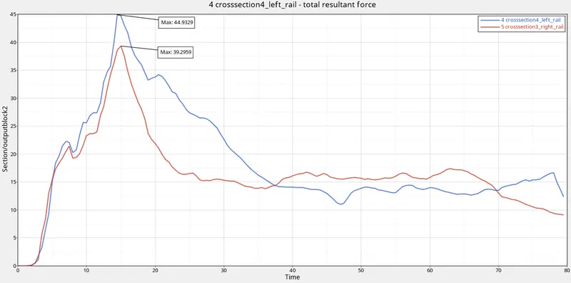
ii) As the Bumper gets deformed completely or reaches its fracture zone the Rail starts absorbing the energy.

iii) The maximum force the rail can take is reached between 10-15ms and then deforms gradually.

iv) The force does not start at T=0 because the bumper is taking all the forces at that time.

v) The left rail can take more force (44.93KN) than the right rail(39.29KN) due to the unevenness on both sides.

3. Shotgun Section Force:

i) The below-shown graph represents the section force obtained on the shotgun:

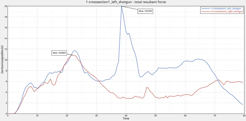
ii) The force does not start at T=0 because the bumper and rail are taking all the forces at that time

iii) The maximum force the rail can take is reached before 40ms.

iv) The left shotgun can take more force (19.97KN) than the right rail(10.89KN) due to the unevenness on both sides.

4. A-Pillar Section Force:

i) The below-shown graph represents the section force obtained on the A-Pillar:

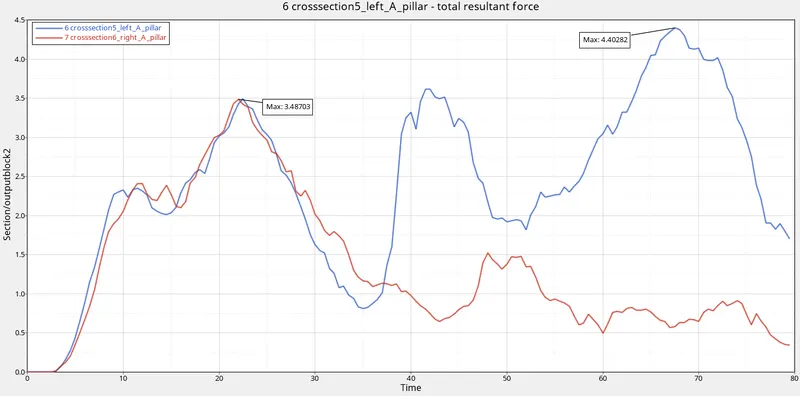
ii) The A-Pillar receives the least force in the system.

iii) The maximum force the rail can take is reached before 70ms.

iv) The left A-Pillar can take more force (4.4KN) than the right A-Pillar (3.48KN) due to the unevenness on both sides.

5. Force Transmission on one side:

i) The below-shown graph represents the forces obtained on the left side of the car:

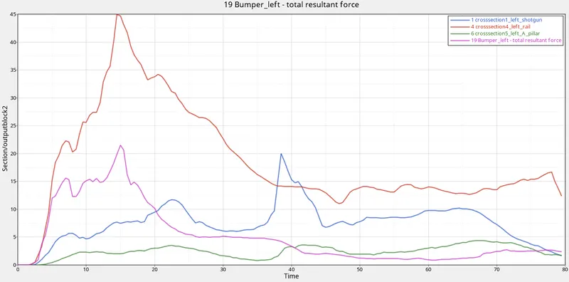
ii) From the graph we can infer that the rail takes the maximum amount of forces.

iii) This is followed by the Bumper and the Shotgun.

iv) The A-Pillar receives the least force in the system.

e) Intrusion on the dash wall:

i) The below-shown graph represents the intrusion on the dash wall measured using springs:

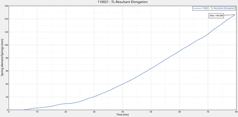
ii) The intrusion observed on the dash wall is 146.5mm which is high.

iii) This is due to the absence of engine components upfront.

iv) Hence all the forces get transferred to the dash wall.

v) With the inclusion of the engine and other sub-assemblies we can reduce the intrusion on the dash wall.

f) Accelerometer Readings:

i) The below-shown graph represents the accelerometer readings on the left and right sides of the B-pillar:

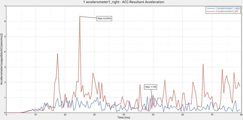
ii) From the graph, we can infer that the left B-Pillar(6.3mm/`ms^2`) experienced a higher acceleration than the right B-Pillar(1.14mm/`ms^2`).

CONCLUSION:

i) The Frontal crash analysis is done on the surrogate model of neon Dodge as the complete model could not be analyzed due to the limitation of the Student version of HyperMesh.

ii) Studied interfaces and their types.

iii) Analyzed the energies generated in the car during a crash.

iv) Obtained the values of the sectional forces at the A-pillar, Shotgun and Rails.

v) Studied the crumple zones and the transmission of energy through different components in the crumple zone.

vi) Due to improper meshing, we came across a few errors that were in the acceptable range.

vii) Analyzed the accelerations the occupants will undergo during a crash.

viii) For accurate results, the analysis must be done on the full-scale model.