Frontal Crash Analysis on a Dodge Neon BIW model using Hypermesh and RADIOSS.

Project-1 Report.

• Aim: To perform the deck set up and run the Frontal Crash simulation of the given Dodge Neon car Model.
  

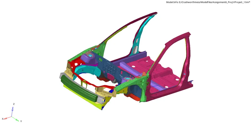
Initial model.

• Objective: 1. To Check for Penetration and Intersections.
  
  2. To create Appropriate Contact Interface wherever needed.
  
  3. To create a Rigid Wall for the simulation.
  
  4. To increase the weight of given model to about 700kg.
  
  5. To give an Initial Velocity of 35mph to the model.
  
  6. To create Sections and measure Sectional Forces across them.
  
  7. To create an Accelerometer on the model.
  
  8. To measure Intrusions on specific locations on the model.
  
  
  
  
  
  
• Procedure:
  
  1. The very first step in the solver deck setup of this model is to check the units in which the Geometry has been modelled. To do this, we need to use the Begin card in the Model tab as shown. Here we can view the basic units of Mass, Length and time that were used in the model.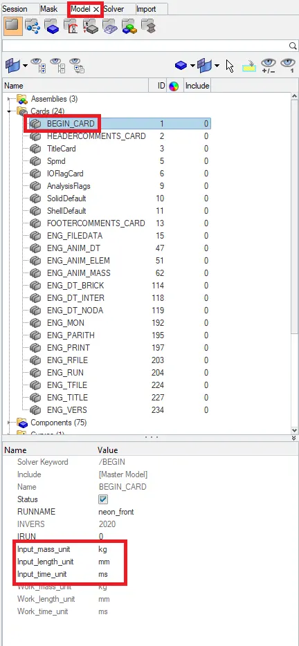
  
  
  
  Begin Card.
  
  
  We can see that the units of Mass, Length and Time are Kg,mm and ms respectively.
  
  
  
  2. After the units were confirmed, we then proceed to check for penetration and intersections in the model. To do this, we simply need to use Hypercrash and use the Penetration checker in the model. We can use this option in the Quality Tab and use the option of Check All Solver Contact Surfaces.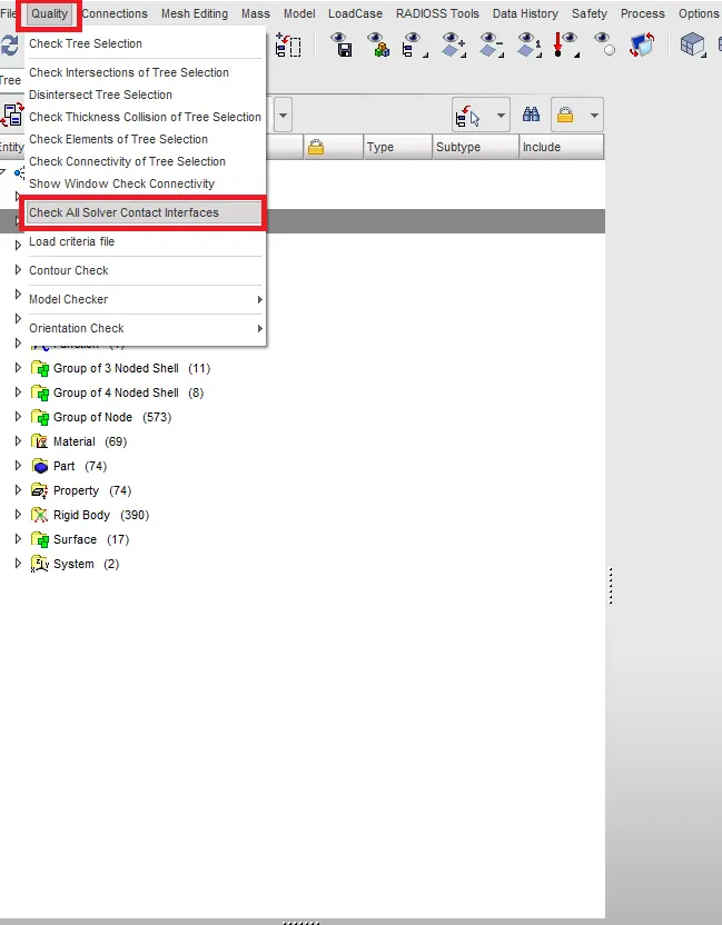
  
  
  
  Quality -> Check All Solver Contact Interfaces.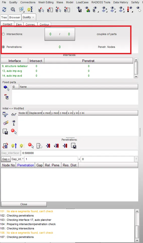
  
  
  
  
  
  Total Intersections and penetrations.
  
  
  We can clearly see that there are no penetrations and intersections in the model.
  
  
  
  
  
  3. After this, we then go onto create a Self impact contact interface. And for this we simply right click in the tree and use the Create New option and use the Contact interface option in it as shown.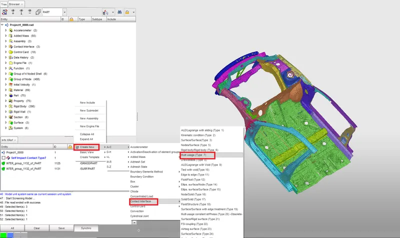
  
  
  
  
  Create -> Type7 contact.
  
  
  
  Like this, we can create a Type 7 contact. Now in this contact we need to define the basic properties such as Igap, Istiff, Inacti etc. We simply change their value to the recommended value.
  
  Here are the recommended values for a Type7 Contact:
  
  1. Istf = 4 (Stiffness based on Softer segment.)
  
  2. Igap = 2 (Variable Gap taken into account.)
  
  3. Idel = 2 (Remove Slave nodes from contact because of element deletion.)
  
  4. Inacti = 6 (Reduce gap by 30% more than the defined gap.)
  
  5. Iform = 2 (Frictional forces are calculated according to the Stiffness parameters.)
  
  6. Stmin = 1KN/mm (Minimum stiffness to avoid a too soft contact.)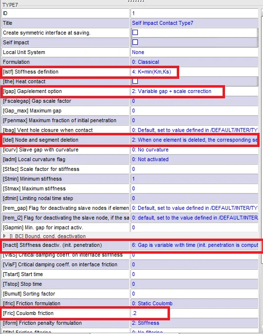
  
  
  
  
  Recommended Properties.
  
  
  Then after this step, we simply need to give in the Slave nodes and the master segment. Since we are defining a Self Impact in the model, the Slave and Master segments for this contact will be the entire given model. So, we then select the slave and master in the graphics area.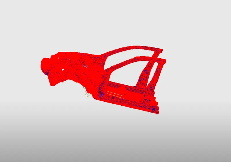
  
  
  
  Self Impact Contact Defined.
  
  
  
  
  4. After this step, we need to check all the rigid body connections in the model. To see if we have appropriate connections defined throughout the model, we need to do it by visual inspection. So, for this, we simply move around the model and check if two surfaces are connected appropriately. Any two surfaces that have a gap between them must be connected using either Rigid Body connections or even springs in some cases.
  In case we get two surfaces, where the contact is not appropriately defined, we then need to add a Rigid body Element or maybe a Spring Element.
  
  
  
  
  
  5. After checking for all the Rigid Bodies in the model, we then proceed to create the Rigid Wall for the Simulation. To do this, we simple use the Create new option that appears when we right click in the Tree. We need to create a Plane Rigid Wall for this simulation.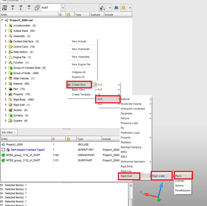
  
  
  
  Create -> Rigid Wall.
  
  
  We then need to edit the properties of the Rigid Wall as following: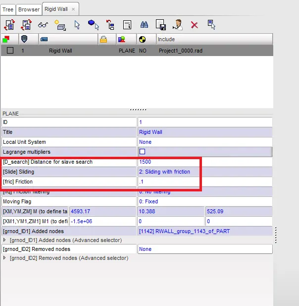
  
  
  
  Rigid Wall Properties.
  
  
  We use the value of 0.1 for friction as requested for this case. The Dsearch distance we can use can be around the range of 1500-2000mm. All the Nodes within this distance will be considered as salve nodes for the contact between the BIW model and the Rigid Wall. We can add seperate set of nodes to this Rigid wall that the system should consider for Slave nodes in the option of [grnod_ID1] as shown. We can use this option and add all the nodes in the model to the Slave nodes.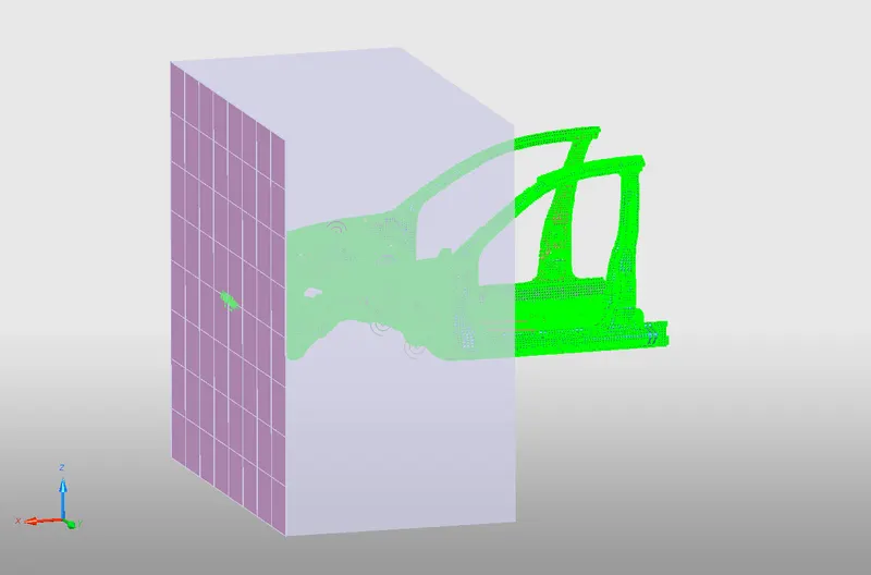
  
  
  
  Rigid Wall Defined.
  
  
  As we can see, the Rigid Wall has been defined and the Green nodes indicate all the Slave nodes that are going to be used in the contact between the Model and the Rigid Wall.
  
  
  
  
  
  6. After defining the Rigid Wall, the next step is to Balance the mass in the model. The current weight of the model is shown to be around 188kg. But since we need to simulate and replicate the whole weight of the vehicle body, we must increase the weight of the given body to approximately 700kg. To do this, we can simply add mass at various points in the model.
  
  The mass to be added is 700-188 kgs = 512kgs. So, we must add this mass to the various nodes in the model. But, while adding mass to the model, we must also change the location of the COG to the desired range (In general, the COG of the body is under the driver). To add mass in the model, we must use the option of Added mass in the Loadcase tab.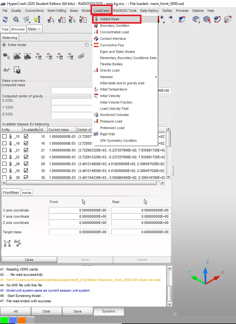
  
  
  
  Loadcase -> Added Mass.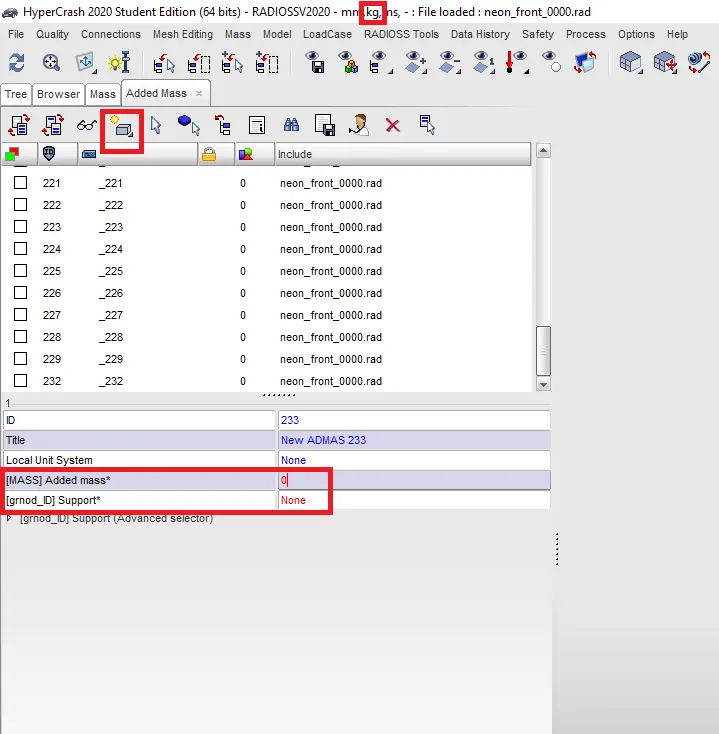
  
  
  
  
  Added Mass command.
  
  
  Before we can add mass on the model, we need to be careful with the units of the mass. When we began the set up of the model, we set the units of mass as kg. We can add mass on the nodes by creating a new object (from the icon shown in the picture above). Then we must add the amount of mass that we need to add, say for example, If we wanted to add the mass of the seat onto the given model. We will then add another 40kgs on the location of the seat. We need to add select that set of nodes in [grnod_ID] and then add this mass. Just like this, we need to add masses into the model and reach the desired mass of 700kgs for the model. We can confirm the total mass of the model using the Mass -> Balancing command.
  
  We can review the CG of the model using the "Show CG point" command as shown below.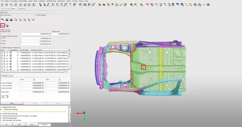
  
  
  
  Initial COG of the Model.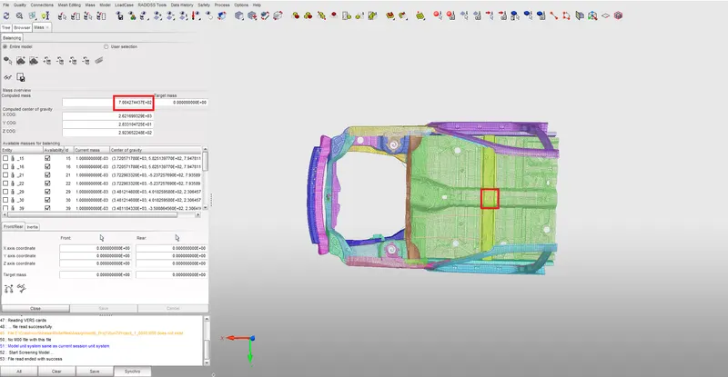
  
  
  
  
  Final COG after the masses were added.
  
  
  
  
  7. After the target mass of the model is reached, then we need to give an Initial Velocity to the vehcile. In our case, we give the initial velocity of 35mph which when converted to mm/ms is around 15.65mm/ms. To give an Initial Velocity to the model, we need to use Initial Velocity tab under the Loadcase tab as shown below.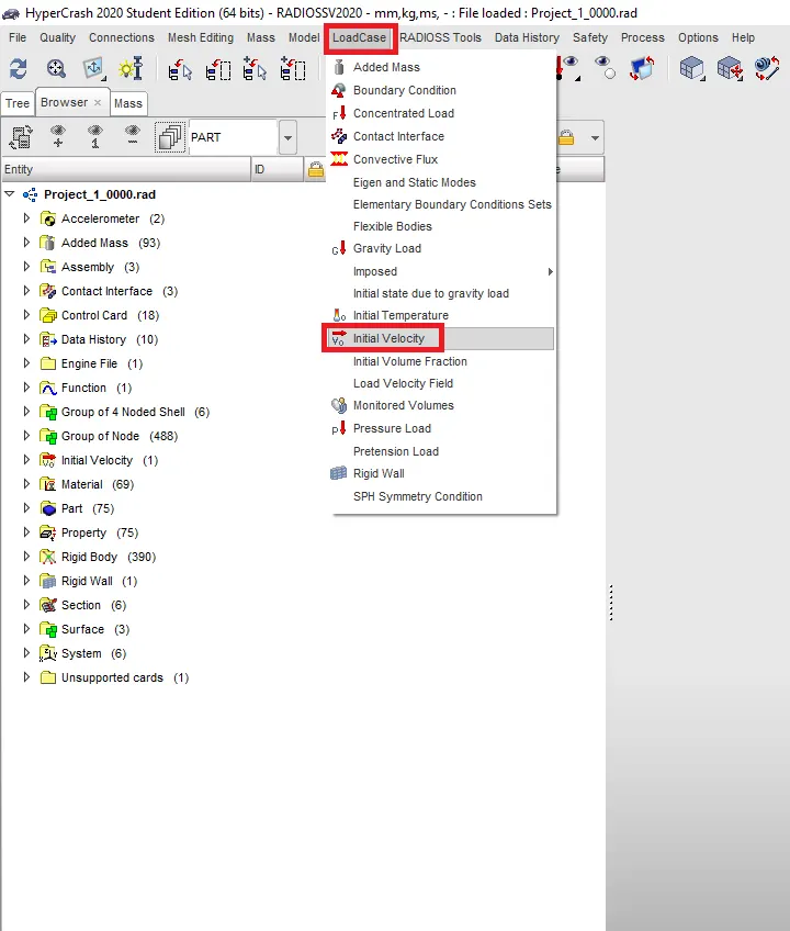
  
  
  
  Loadcase -> Initial Velocity.
  
  
  After we need to select the Direction and the Nodes on which the Initial Velocity is needed to be applied. For our setup we give the magnitude as 15.65 mm/ms and as for the nodes, we need to select the entire body of the vehicle.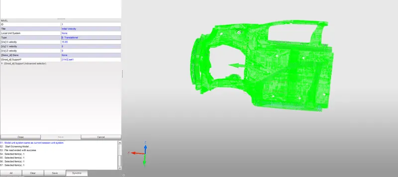
  
  
  
  Initial Velocity applied with properties.
  
  
  
  
  
  8. The next step after giving an initial Velocity to the model is create sections to study the sectional forces at specific areas or parts of the model. So to make sections in the model, we need to create a skew to define the section. So, to find the node with nodes Id 174247 as asked, we need to create a temporary node on it. To make a temporary node, we can use the shortcut of Shift+F2. We then need to right click on nodes and select the option of "by ID" as shown below:
  
  
  
  Creating Node by ID.
  
  
  We then enter the node ID and then click on add. A temporary node will be made on the node that has an ID of 174247. We then go and mark this node and further go ahead and define sections on it. So, to define a section, we need to define a Skew first. To define a skew, we simply need to right click in the tree and select the option of Skew. We must select three nodes that will then go on to define the three axes of the Skew system that we are creating.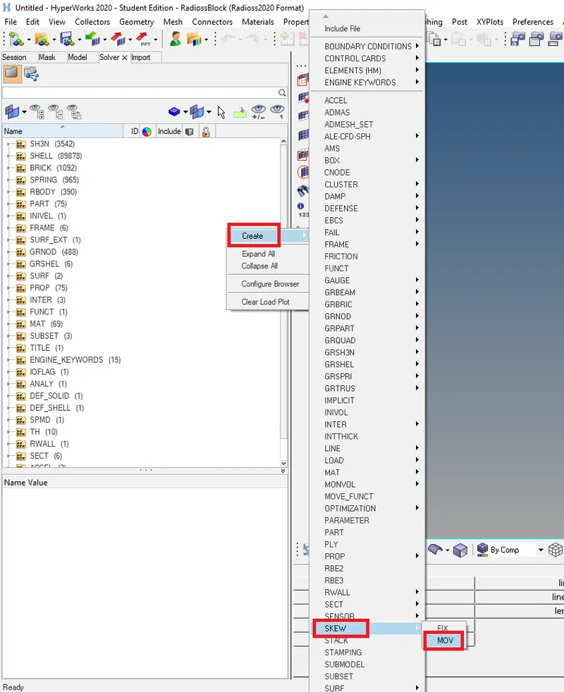
  
  
  
  Create -> Moving Skew.
  
  
  We then need to select the three nodes on which we need the Skew system. In our case setup, we need to define around 6 sections. We need to make sure that the normals of all the sections defined need to be in one particular direction. All the normals can be facing either the wall or even away from the wall.We need to make sure that they are in a single direction.
  
  We can create a Section just in the same way as we created a skew system. We need to right click in the Tree and select Sections as the following: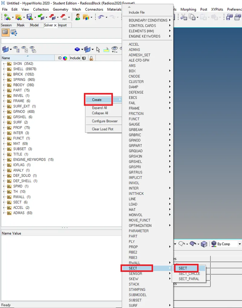
  
  
  
  Create -> Sections.
  
  
  After we define a Section, we then need to give the input of all the elements for the definition of the sections. We need to define a section and give in the three Nodes and also the elements on which we need to make the section on.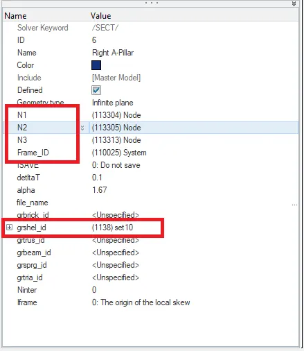
  
  
  
  Sections Properties.
  
  
  In the grshel_id we need to select the elements on which the section is to be defined. We must also specify the Frame ID for the section. Similarly we can define all the Sections in the model.
  
  We make sections in the model so that we can study the peak forces at those particular sections. All the Sections were defined as the following: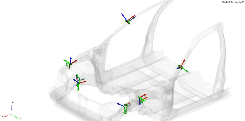
  
  
  
  All the defined Sections.
  
  
  We can clearly see that the Normals for all the Sections defined have a similar direction, i.e. away from the Wall.
  
  
  
  
  9. The next step is to setup a Contact Interface between the Bumper and the Components near it to study the Axial Forces received on the bumper from the wall. We can set up the Contact in the similar way as we set up the Type7 self impact contact on the vehicle. We need to select the Master as the Bumper and the Slave segment as component behind it. The final defined Contact interface can be seen as the following: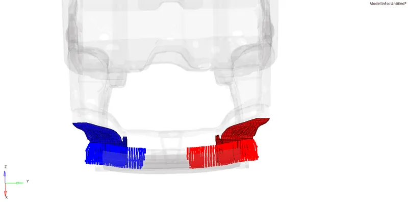
  
  
  
  
  Bumper Type7 Contact Defined.
  
  
  We can then request the Contact Interface Forces in the Time History Plot that we will plot later.
  
  
  
  
  10. The next step is to create an Accelerometer at base of B pillar in the model. An accelerometer is an electromechanical device used to measure acceleration forces. Such forces may be static, like the continuous force of gravity or, as is the case with many mobile devices, dynamic to sense movement or vibrations.
  
  To add an Accelerometer to the model, we simply need to right click in the tree and select the Create option and use the Accelerometer in it.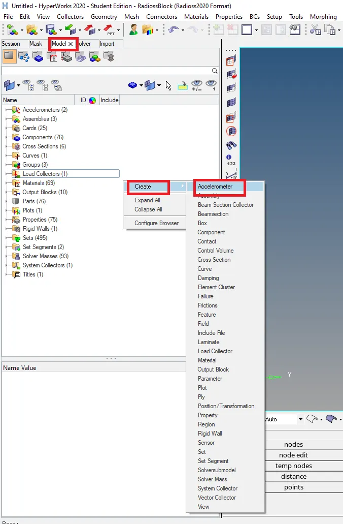
  
  
  
  Create -> Accelerometer.
  
  We then need to specify the Node on which we want the Accelerometer to be. In our case, since we need the Acceleration at the base of B-pillar, we place the Accelerometer at one of the nodes under the B-pillar in the main body.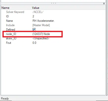
  
  
  
  Node for Accelerometer.
  
  
  In node_ID we can give the node below the B-pillar. We need to create two separate Accelerometers for two different nodes under the B-Pillar in the model.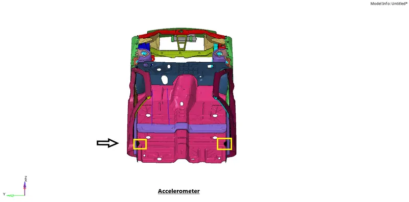
  
  
  
  Accelerometer Defined.
  
  
  
  
  11. In the next step, we will create a spring to measure intrusions at the given node ID's: 66695,66244. Then we will create a spring between nodes 66695 and 121739 and nodes 66244 and 122048. We need to create Springs with a low coefficient of Stiffness so that we can measure the intrusions on that node and see how the node behaves under the forces that are being acted upon it. We can locate the required nodes in a similar manner in how we located the node to measure the sectional forces. We simply used the temporary node command and used the by ID option.
  
  When these nodes are located, we then need to create a Spring element between them. To create a Spring element between the nodes we can use the Springs option under the 1D tab.
  
  
  
  1D -> Springs.
  
  
  
  
  Springs command.
  
  
  Here we need to select the two nodes and then the Spring element is created. After the Spring element is created, we then need to assign a property to it. To assign a property, we simply create a property and then assign this property to the spring.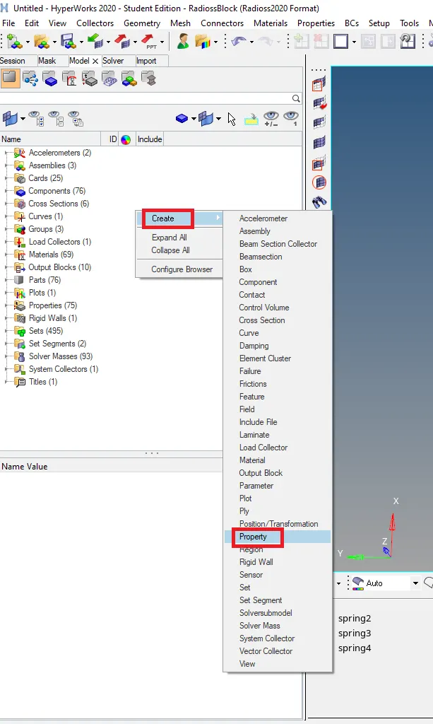
  
  
  
  Create -> Property.
  
  
  We need to change the property card to Spring4 and give a very low value for the spring mass and Spring constant as shown below: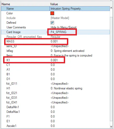
  
  
  
  Spring Properties.
  
  
  Then after the spring property is created, we then go on to assign this property to the spring component. To assign property to the spring component, we simply need to right click on the componentand use the Assign option.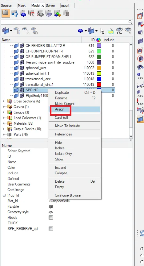
  
  
  
  Assigning Properties.
  
  
  Like this, the property for the spring is succesfully assigned to the component.
  
  
  12. The next step is to give the Timestep for the simulation. There are various cards that we need to add and give different values for them. For example: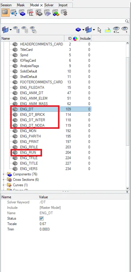
  
  
  
  ENG_DT values are shown in the snapshot above.
  
  ENG_RUN has a value of 80.0ms.
  ENG-DT-BRICK- Tscale:0.9, Tmin: 0.0001ms
  ENG_DT_INTER- Tscale: 0.67, Tmin: 0.0003ms
  ENG_DT_NODA- Tscale:0.67, Tmin:0.0001ms
  
  All these values will affect the simulation time and the results we get.
  
  
  
  13. One of the final Steps in the Deck setup of this simulation is to request a Time History(TH) File from the Solver. So to create a Time History File we simply need to right click on the Solver tab and use the create option. Under this option, we will have another option of TH. Under this option, we can request a certain TH output.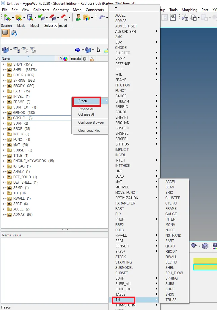
  
  
  
  Create -> TimeHistory (TH)
  
  
  For example, if we have to create a TH for the Accelerometer that we have setup, then we will need to use the option of ACCEL under the TH command. When we make this TH, we then need to give the two accelerometers and then this TH file is setup.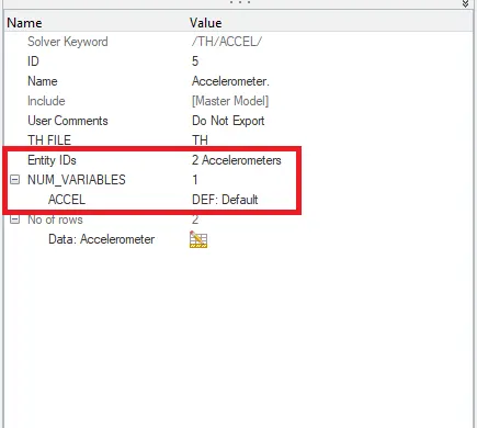
  
  
  
  TH For Accelerometers.
  
  
  We can edit the Number of variables and request specific Outputs of certain components. These outputs can be Acceleration, Displacement, Velocity etc.
  So similarly, we can setup all the TH files as required in our case study. The following TH files were requested: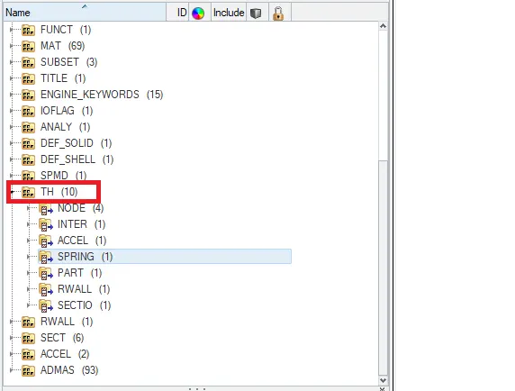
  
  
  
  All TH Files Requested.
  
  
  
  14. After the Deck Setup is done, the last step includes checking the model in the Model checker. To check the model, we can use the Model checker in either Hypermesh or Hypercrash. In Hypermesh, the Model checker can be accessed under the Tools tab.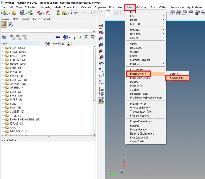
  
  
  
  Tools -> ModelChecker.
  
  
  This model checker will show all the warnings and errors in the model. All the errors must be resolved and the warnings if not critical, can be left in the simulation, else, they too must be resolved. Like this the model can be checked and be resolved for any errors in the model.
  
  After the model checker is run, we then go on to run the simulation. To run this simulation we have to use the Radioss command in the Analysis tab.
  
  
  
  Analysis -> RADIOSS.
  
  
  
  
  RADIOSS Command.
  
  
  The input file is the file location in the system where we want to save all the simulation files, such as the .h3d file and the T01 files for example.
  
  After the simulation is run, we can confirm that the simulation has run properly when we see a NORMAL TERMINATION at the end of the simulation as follows: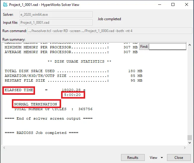
  
  
  
  Normal Termination and Elapsed time can be seen after the simulation is completed.
  
  
  In this, we can see the Elapsed time as well. In our case, it is around five hours and twenty seconds.
  
  We can then later view the simulation in Hyper-view or by simply clicking on Results.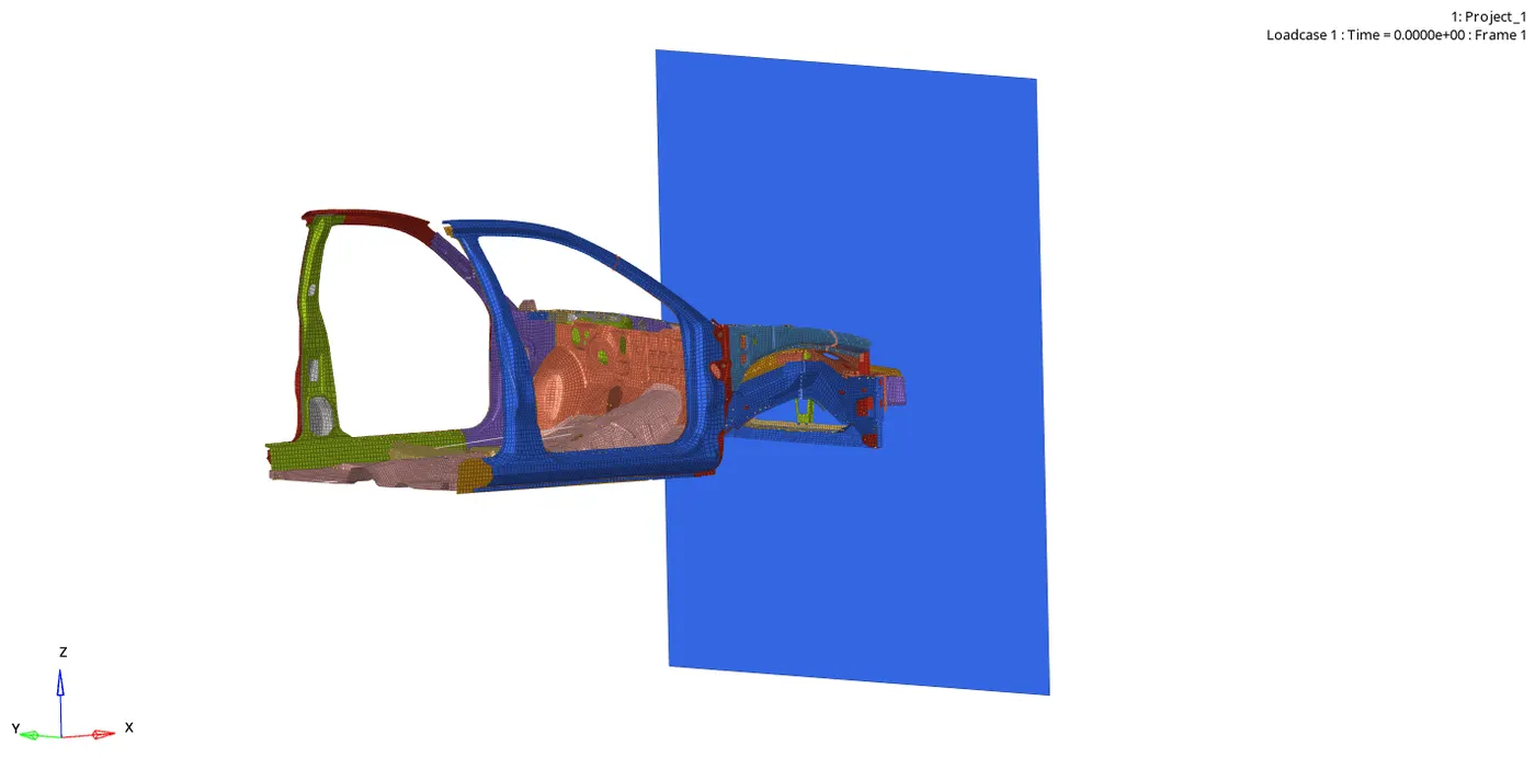
  
  
  Animation of the simulation.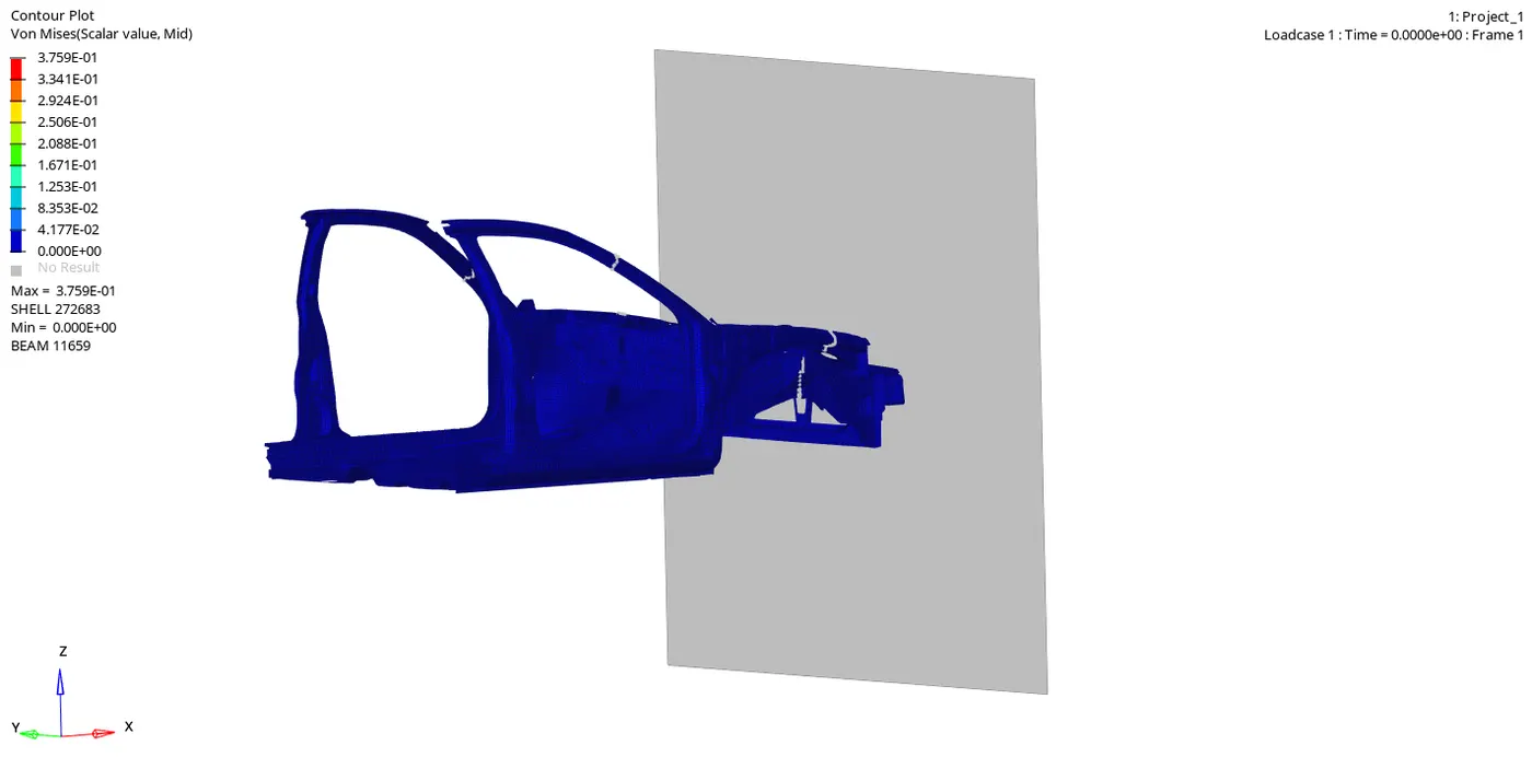
  
  
  
  Von-misses Plot.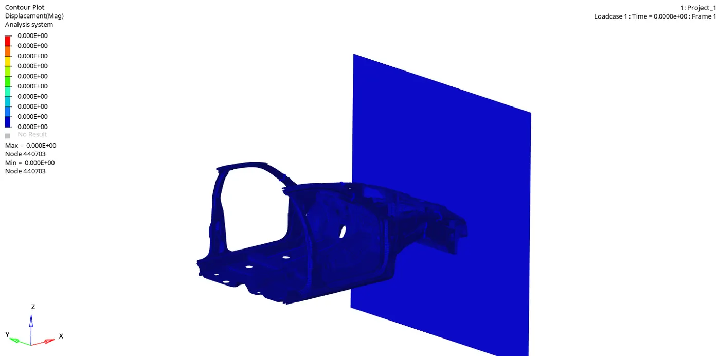
  
  
  
  
  Displacement plot.
  
  15. The very last step is to study the Simulation results by plotting all the necessary graphs and extracting data from them. To plot graph, we need to use the Hypergraph tab. To access the Hypergrraph tab, we simply need to change as the following: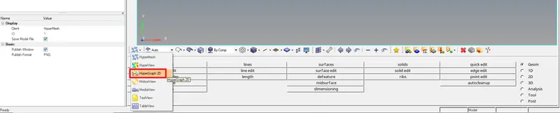
  
  
  
  Hypergraph 2D
  
  In this tab we need to open the Time history file. It is the T01 File that will be available in the Folder where we saved all the files. We can import this file by clicking on the icon shown below:
  
  
  
  HyperGraph Command.
  
  
  We can set the variables between which we need the graph to be plotted as well.
  
  
  A. Sectional Forces in the model.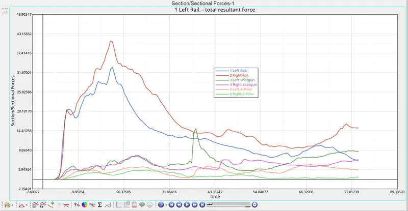
  
  
  
  Sectional Forces Plot.
  
  
  All the Sectional forces have been plotted in the graph shown above. We can clearly see that the Right hand Side Rail of the BIW has a higher peak than the Left hand side Rail. This can indicate that the Right side Rail is experiencing a much greater force than the Left hand side Rail. After the Rail, the forces are transferred onto the Shotgun. Since the right rail had absorbed a much greater amount of force, the right shotgun has a relatively low amount of force to absorb. Similarly in the case of Left Rail and the Left Shotgun. Since the Left Rail aborsbed a relatively low amounts of forces, these forces got carried onto the Left Shotgun. And now, the Left Shotgun will have a much greater amount of forces to abosrb. This can be confirmed by the peak of the two graphs, i.e of the Left and the Right Shotgun. We can clearly see that the Left shotgun has a higher peak than the Right Shotgun.
  
  The rail will collapse before the shotgun because it is in the normal direction to the Rigid Wall. The Rail behaves like a first Point of contact when the crash is occuring. Whereas, the Shotgun will receive forces after the Rail.
  
  
  
  B. Energy Plot.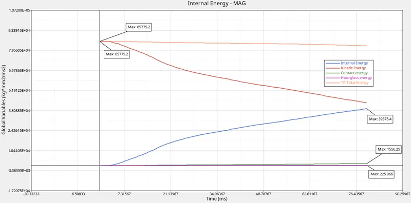
  
  
  
  
  Plot of various energies in the simulation.
  
  
  
  Ideally: `("Hourglass Energy"+ "Contact Energy") / ("Total Energy") <= 15%`
  
  In our case:
  225.966+1556.25 / 85772 = 2%
  
  This means that the above condition is satisfied.
  
  
  From the Above plot, we can see that the Total Energy is decreasing by a little margin and that the contact energy is also minimal. We can observe that the Total Energy has peaked out at 85,775.2J and the Hourglass Energy has a peak of 225.966J. We can clearly see that the Kinetic Energy is being converted into Internal energy. Ideally all of KE should be converted into IE and the Total Energy must remain constant, but in our case since we have Hourglass Energy error, our Total Energy is decreasing. We can rectify this hourglass energy by further reducing the Timestep of the simulation and giving the Ideal Properties wherever we can.
  Our Requirement from an Ideal Simulation is that we have minimal Contact energy and maximum Energy absroption/Deformation in the elements. We can check the Energy error in the Engine output file, which has maxed out at -2.1% which is within the appropriate limits for it to be. Our Mass error is also 0.0% which means that the solver did not need to add mass onto the nodes to reduce the timestep to further avoid the Hourglass Error.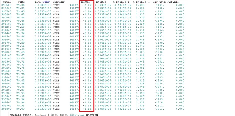
  
  
  
  Engine File Output.
  
  
  
  
  
  C. Accelerations recorded on the Accelerometers.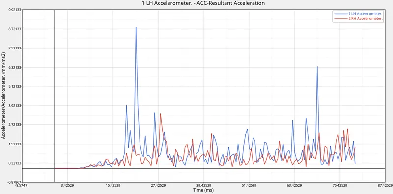
  
  
  
  Acceleration Plot
  
  
  From the Plot above, we can see that the Peak acceleration of the Left hand Accelerometer is much much higher than that was recorded on the Right hand Accelerometer. This is because of the displacements on that side of the model and it can be confirmed by the simulation. The peak of the Left hand Accelerometer was somewhere at 8.7 mm/`ms^2` and whereas the Right Hand Accelerometer peaked at 3.5mm/`ms^2`
  
  
  
  
  D. Intrusions on the Spring element:
  
  
  
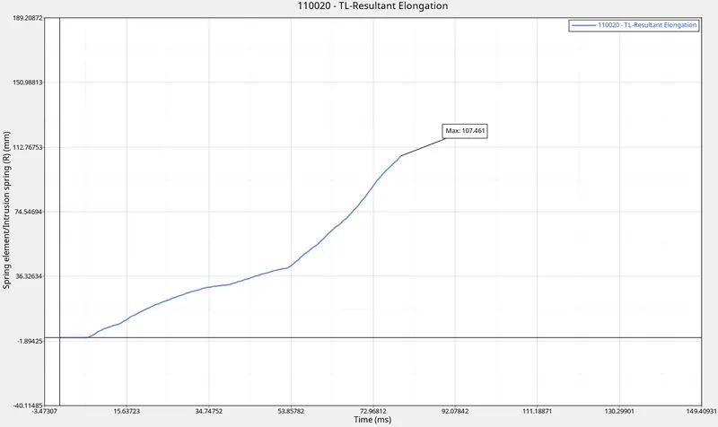
  Spring1 Elongation.
  
  
  
  
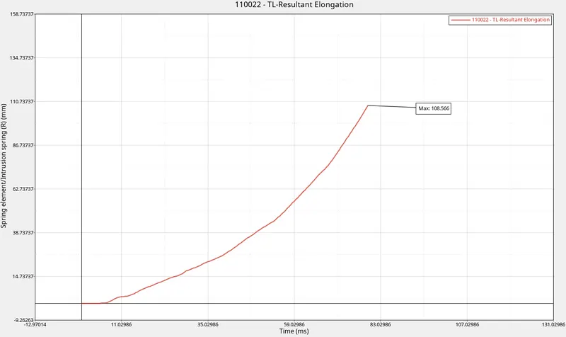
  Spring2 Elongation.
  
  
  The total Elongation on the two springs have been plotted. The first spring has an Elongation of 107.5mm and the second spring has an elongation of 108.6mm.
  
  
  
  
  E. Axial Forces on the Bumper: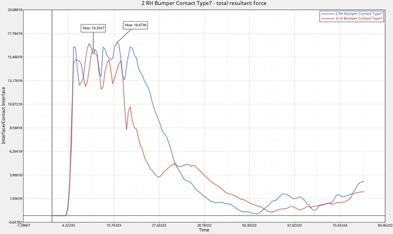
  
  
  
  Axial Forces on the Bumper.
  
  
  Total Resultant Force on the Bumper contact can be seen. We can see that both the curves are pretty similar and conclude that the crash is almost alike on both the sides of the model. The curve drops earlier in the left hand of the bumper meaning that this side is failing earlier than the other. The Right hand Bumper contact interface has peaked out at approximately 16.9KN and the left side has peaked out 16.36KN.
  
  
  
  
  
  
  
  
  
  
  
  
  
  
  
  
  
• Conclusion: In conclusion, I would like to state that this project helped me get a proper understanding on the procedure of doing a Frontal Crash of a vehicle and how to extract different data from the simulation.