Assignment 5-RADIOSS Interfaces & Study of Effect of Notches Challenge

Assignment 5

RADIOSS INTERFACES & STUDY OF EFFECT OF NOTCHES

Aim: To mesh the bumper component with target element size of 6mm and also doing a study of RADIOSS interfaces and effect of notches, by simulating the crash tube component.

Objective:

• Perform geometrical cleanup on the bumper and mesh the bumper with target element size of 6mm
• Run the crash tube model with or without changing the parameters

Parameters that need to change during simulation of crash tube

• Run the crash tube model as it is
• Change the inacti = 6 and run
• Create the type 11 contact and run
• Remove both notches and remove boundary condition on rigid body node and then run
• Create a new notch on the middle of crash tube and then run the model
• Create a new notch with nodes only from opposing two faces and run

Given by Technical Support team

Meshing of Bumper component

Procedure:

Import the model as in Hyper-mesh by using import option

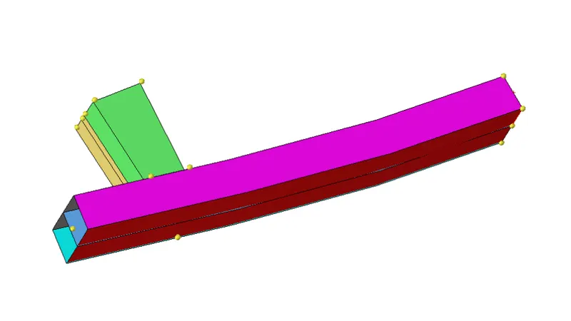
Bumper of car

• After importing the model, the first step is to check the geometry whether there is any error present in the geometry or not for that switch to 2D Topo modo to visualize the geometry.

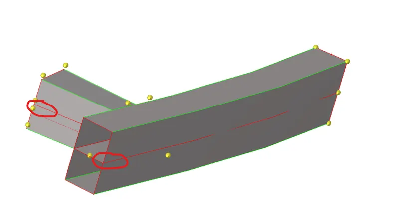
Free edges in the geometry

• As you see here red colored edges, these are basically free edges, means edges which are not connected to any surface, but here these free edges are basically a geometrical error we need to fix them, for that we using surface extend option.

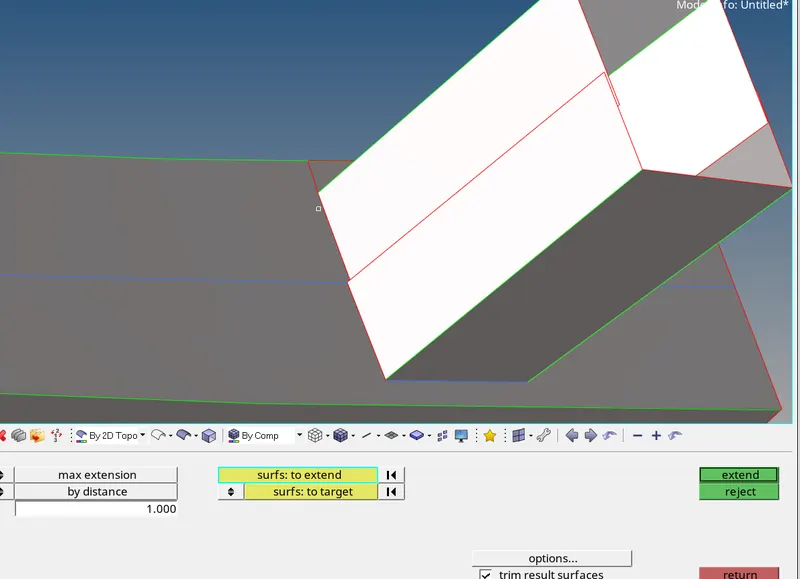
• In surface extend option select the surface which need to extend and then select the target surface up to which the surface is extended, also make sure to check out the trim result surfaces, so that surfaces may not intersect with each other.

• Also, there is lot of error present in the geometry which we need to clean, we can either clean it manually or either we can use the auto-cleanup option to clean the geometry, removing all the unwanted surface and clean the geometry.

• After cleaning the geometry, the next step is to mesh the component, for that go to 2D Panel > Auto-mesh option, set the target element size = 6 unit and then select the surface that need to meshed.

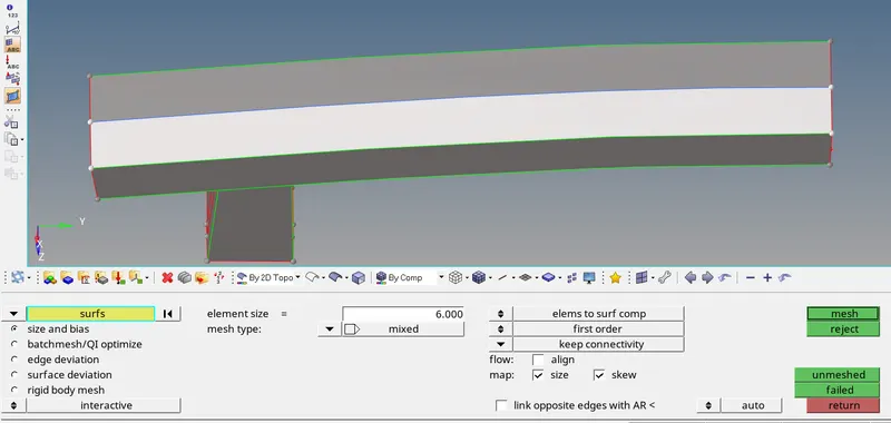
Meshing the component with Target element size of 6 unit

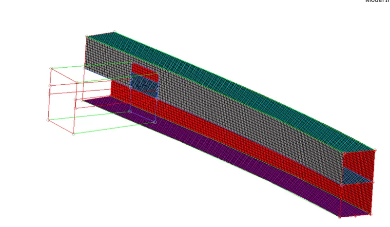
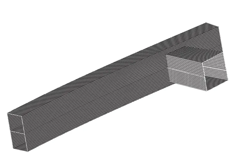
Meshing of the Bumper

• After meshing the bumper, now we can also reflect that to create the other half side of the bumper.

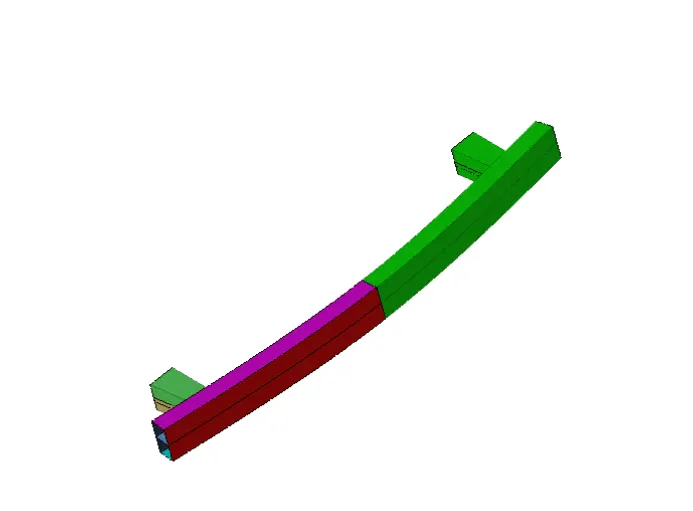
Reflection of Bumper part

• Here we reflect the bumper in the same component that we created, but we need to move the bumper part to their respective component where particular material and property is assigned to it. To move the parts to the respective component we use the organize option to move the parts to their respective component.

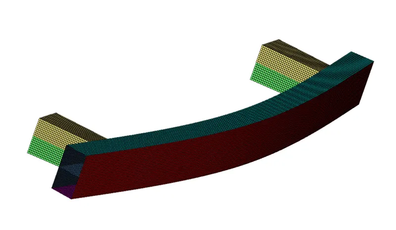
Meshed model of Bumper

What is Interface modelling

• Explicit analysis solves highly complex nonlinear problems and contact plays an important role
• The accuracy of these result depends upon the accuracy of the interface modeling.
• The interfaces are defined through master and slave segments
• The algorithm takes the master and slave segments and checks for initial penetration between slave and master, This checking is done at every time step
• The master and slave selection can be of parts elements nodes etc.

Most widely used contact algorithms are

Type 7, variable stiffness node to surface contact

Type 11, variable stiffness, edge to edge contact

Interface type 7 Node to surface contact

• It is node to surface contact and it is a universal type contact
• A gap is defined around master and slave nodes and this gap can be variable or constant
• The slave is kept outside of the master gap by resistive force application

Advantages:

• The type 7 interface is non oriented and slave nodes cab belong to master surface unlike type 3 and type 5
• The search of master and slave segment is carried out using a direct search algorithm.
• Energy jumps because of edge impact are removed by cylindrical gaps around edges
• Has variable stiffness and stiffness is not constant throughout, due to this instability because of node penetration through thickness is removed

Disadvantages

• Require more stringent modelling practice
• Don’t tolerate intersection
• Time step may reduce due to increasing interface stiffness

Important Parameter of Type 7 contact interface

Interface Time step

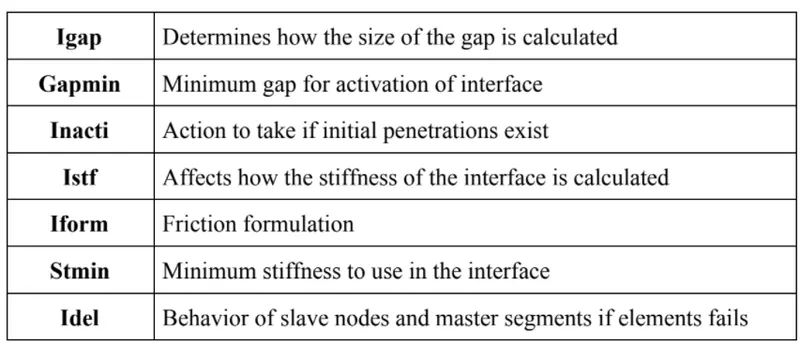
• As the stiffness is non-linear the slave node can’t cross the master segment, this imparts greater accuracy while solving
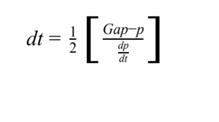
• However, this means that interface time steps need to be evaluated during the solution. If there is large penetration the interface stiffness become large leading to reduced time step.

The interface timestep can be calculated as below

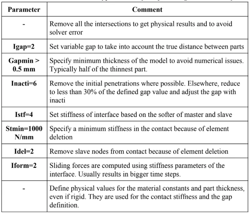
Recommended properties for Type 7 contact

Limitation of Node to Surface Interface

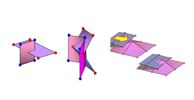
There are the situations where TYPE7 interface node to surface will not detect the contact due to edge crossing each other at an angle. TYPE11 contact can be added to capture physics properly.

Source: Altair

Type 11 Edge to Edge contact

• One of the drawbacks of type 7 contact is that it cannot remove the element intersection that is present in the model
• This interface simulates impact between edge to edge or edge or lines. A line can beam or truss element or a shell edge spring element. In association with interface TYPE7, TYPE11 solve the locking cases.
• Defined by identifying master and slave lines (edges)
• Impact occurs between a master and slave line. A slave line can impact on one or more master lines, a lime can belong to the master and slave side, this allows self-impact.
• To avoid that kind of issue and edge related intersection Type 11 contact is preferred.
• Type11 work very much similar to the type 7, but here search is only for the edge of the model.
• Used mathematical complicated algorithms therefore, it is strongly advised to used it only when necessary. A huge interface TYPE11 can slow down computation.
• The recommended parameters are the same as that of type7 interface.

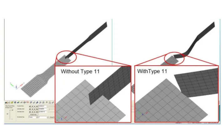
With & Without Type11 contact

Source: Altair

TYPE19 interface (combination of Type7 and Type11)

• Combination of two symmetric TYPE7 interface and one TYPE 11 interface
• Common input based on same slave and master surfaces.
• Useful for complex contact problems such as airbag unfolding
• Computationally expensive so only problematic segments should be defined
• Edge to edge contact flag ledge

PART 2

Import the starter file into the solver deck RADIOSS

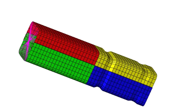
Crash tube

Case 1: Run the crash Tube as it is

• Before running the simulation, we have to create the TH for the interface, and it should be follows for all the cases.
• To create TH. Go to solver Browser >> Right click on TH >> create >> INTER

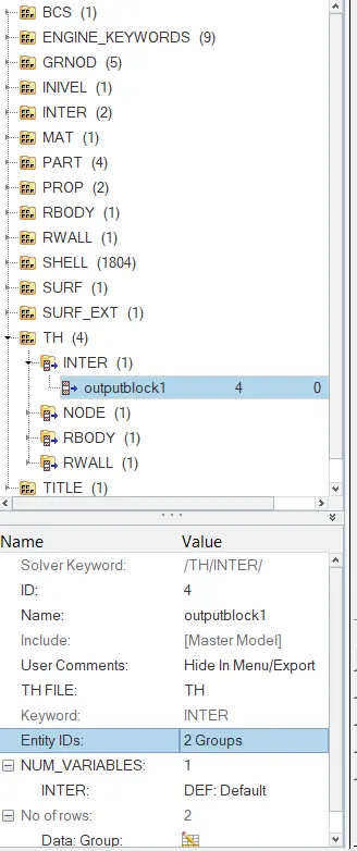
• After creating TH. The contact interfaces should be assigned to that I.e. Seam weld (TYPE2) & Self contact (TYPE7)

Default parameters

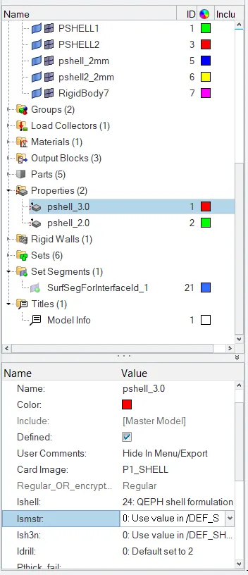
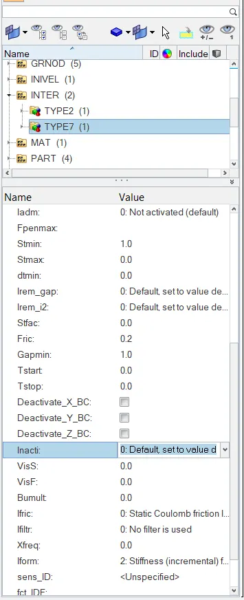
TYPE 7 contact is defined

• Now we can run the simulation, for that go to Analysis panel >> RADIOSS >> select the input file >> save it in different folder and name it >> Run, also setting the -nt 3, whereas nt is number of threads or number of cores used to solve the problem.

• After completing the simulation, the RADIOSS will popup a solver window stating RADIOSS job completed, which indicates simulation has been finished, also showing the total number of cycle and Elapsed time, means time required to solve the problem.

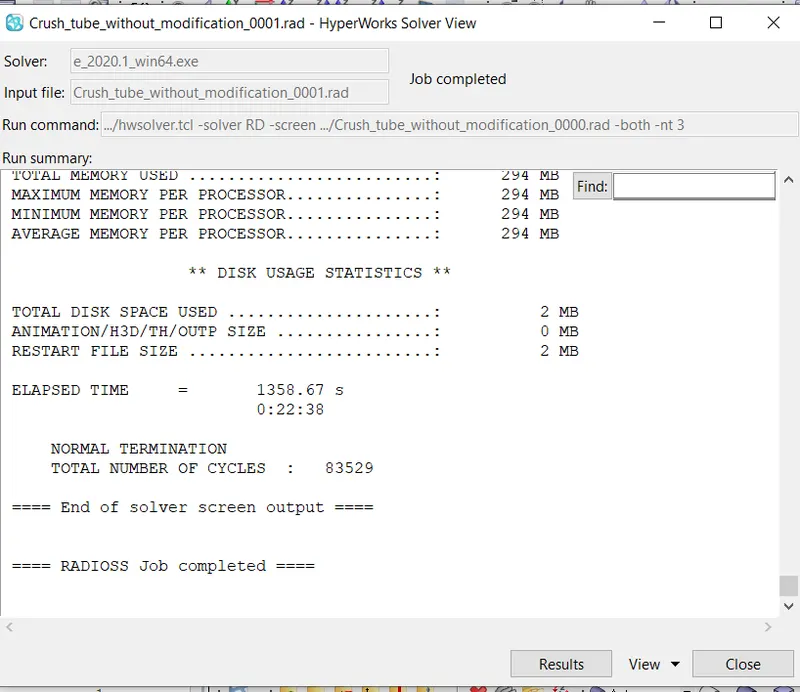
End of solver Output

• After running simulation animation files will be generated where we specified a location to store the file

To check the value of Energy error and Mass error, open the 0001.out file in Note pad

Energy error:

• If energy error is negative, it means some energy is dissipated. This dissipation can be of any type for example in case of under-integrated elements, the Hourglass energy can explain a negative energy error since it is not counted in the energy balance. The acceptable amount of Hourglass energy is about 10-15%
• If energy error is positive there is energy creation. In case of QEPH elements the solution is calculated accurately as there is no hourglass energy is produced. A positive energy error of 1-2% is acceptable.
• If energy error is -99% the computation has diverged, this happen due to false energy balance that is created due to improper model definition.

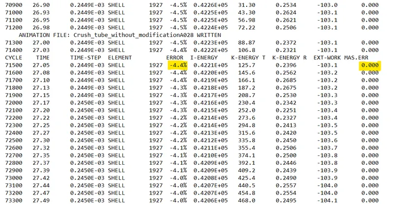
Here we no mass error and energy error is -4.4% which is under acceptable range

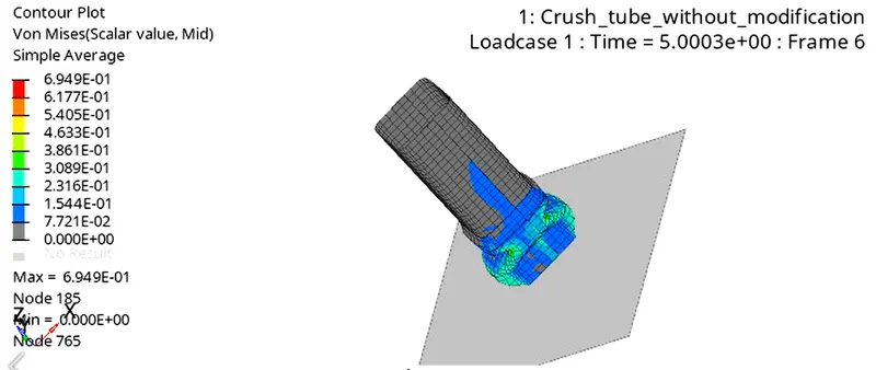
• After that we need to visualize it. For that we need to switch to the Hyper-view utility, in hyper-view we need to import the h3d file that was generated during solving. Now to display the result we need to select the result plot we required, here we check von-misses contour by selecting Global variable as Von-misses, and here we use averaging method as simple to visualize the result.

• To plot the graph, we need to switch to the Hypergraph 2D. we can switch to it using the same client selector option in toolbar, also in single window we can split it into number of windows, where we can plot the different plots. To plot the graph, we required the T01 file to upload to see the graphs. This file is available in same directory where we have .out files, h3d files, here we can plot different graphs like Rigid wall forces, Internal energy, Kinetic energy, Hourglass energy, Total energy to compare and visualize the result.

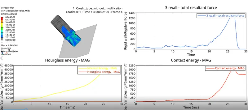
Rigid wall force / Internal energy and Kinetic energy / Contact energy

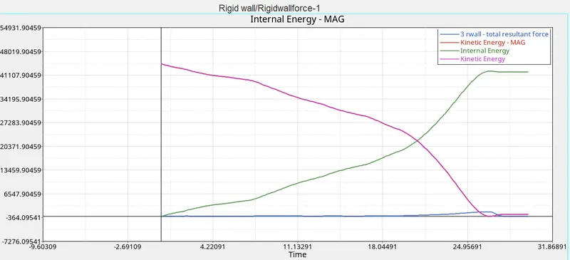
Kinetic energy / Internal energy / Rigid wall force

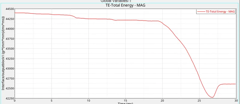
Total Energy

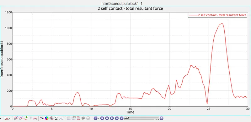
Total contact energy in the global parameter which shows the force transmitted by the contact.

• From graph as you see that rigid-wall force is starting from lower value because initially there is no contact between crash tube and rigid wall.
• There is rise and fall in the graph is because of deformation of crash tube, as the component start bend the rigid-wall force start decreasing, after completing on bend resisting forces start increasing because of initiation of new bend, and when bend will start again there is drop down in the resistive forces. So, these up and down in the curve is nothing but the graphical representation of bend in the crash tube.
• Here Contact forces are initially small because there is no contact occurring initially, and with time deformation start increasing and due to this contact between element increase either it is self-contact or it may be contact with wall both increases with time lead to increase in the contact energy and also the force transmitted by the contact.
• Here as you see the kinetic energy is high at initial level because at initial level velocity is high, and with time velocity and kinetic energy will reduce due to deformation and energy absorbed by the crash tube, so this is the reason of why internal energy is increasing as deformation increasing.
• Here also Hourglass energy is constant and remain to Zero, it means there is no Hourglass effect produce in the simulation, it is because of using the Ishell = 24 (QEPH element formulation with improved integration scheme with Hourglass control)
• Total energy is sum of kinetic energy + contact energy + Hourglass energy + Internal energy. Here Total energy is start increasing from higher value because at initial except kinetic energy all the energy is almost zero so kinetic energy is only there, so total energy now become equal to Kinetic energy, at initially kinetic energy start increasing due to this total energy is high at initial level and it slightly decreasing due to -3.8% of energy error.

Note: Here in this case Type7 contact is defined which is general contact that is used during impact or crash scenario. But here the Inacti = 0 is defined, it means it simply ignore the initial penetration.

Case 2: Change Inacti = 6 and run

• Here in this case, we have to only change the parameter inacti = 6 and rest of parameter keep it as default value.

Now to define the value of inacti = 6, go to Solver Browser > INTER > TYPE 7, here define the inacti = 6

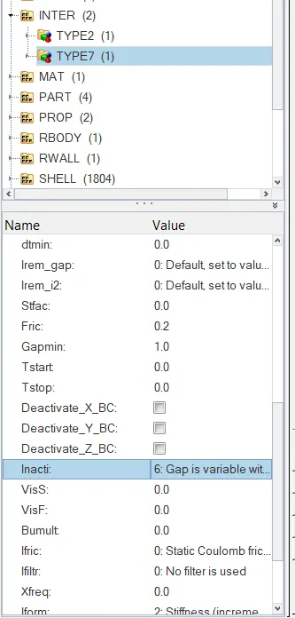
Defining Inacti = 6

• After defining the value of Inacti =6 now we have to run the simulation and save the file name as case 2 and click on RADIOSS to run the simulation.

• After completing the simulation, the RADIOSS will pop-up a solver window stating RADIOSS job completed, which indicates simulation has been finished, also showing the total number of cycle and Elapsed time, means time required to solve the problem.

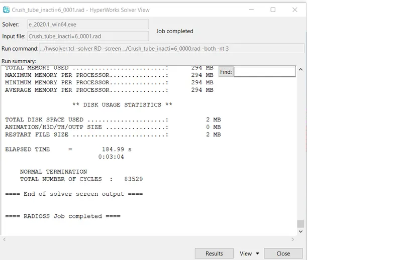
End of solver screen output

Total number of cycles = 83529

Elapsed time or time taken to solve the problem = 184.99s

• After running simulation animation files will be generated where we specified a location to store the file

To check the value of Energy error and Mass error, open the 0001.out file in Note pad

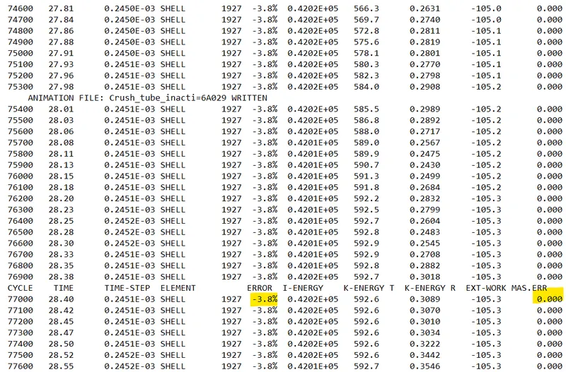
Here the Mass error is 0 or we can say negligible where as the energy error is -3.8% which is in acceptable range

• After that we need to visualize it. For that we need to switch to the Hyper-view utility, in hyper-view we need to import the h3d file that was generated during solving. Now to display the result we need to select the result plot we required, here we check von-misses contour by selecting Global variable as Von-misses, and here we use averaging method as simple to visualize the result.

'

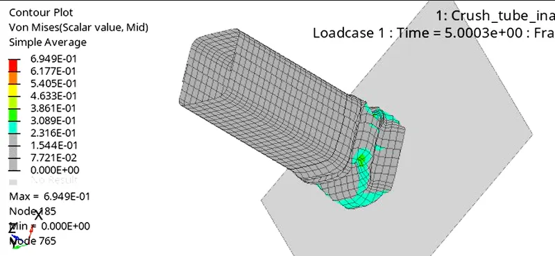• To plot the graph, we need to switch to the Hypergraph 2D. we can switch to it using the same client selector option in toolbar, also in single window we can split it into number of windows, where we can plot the different plots. To plot the graph, we required the T01 file to upload to see the graphs. This file is available in same directory where we have .out files, h3d files, here we can plot different graphs like Rigid wall forces, Internal energy, Kinetic energy, Hourglass energy, Total energy to compare and visualize the result.

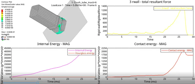
Rigid wall force / Internal energy / Contact energy

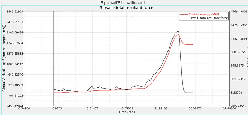
Rigid wall force / Contact energy

• Here we only change the one parameter that is, we define the Inacti = 6, Inacti flag means the initial action need to taken if initial penetration existed. Here if initial penetration is exist, then gap is reduced and scale to avoid penetration. And all we know that Type 7 is very sensitive to initial penetration, but here in above two case there is no initial penetration exist, due to this we got the same result, with little bit fluctuation, here the energy error is about -3.8% which is less as compared to previous case.

• So, it is important to define the proper value of Inacti, because initial penetration in the model, makes the model weak and gives out undesirable and unrealistic results. These kinds of issues are very much simulation setup based and it doesn’t happen in real life. To avoid these issues, the model setup must be proper. The initial penetration will weaken the overall model, To avoid these kind of errors and unrealistic result, the model will be first check for the penetration and intersections, Both kinds of component wise and contact wise penetration and intersection must be checked and it must be removed.

Case 3: Create the Type 11 contact and run

Type 11 Edge to Edge contact

• One of the drawbacks of type 7 contact is that it cannot remove the element intersection that is present in the model
• This interface simulates impact between edge to edge or edge or lines. A line can beam or truss element or a shell edge spring element. In association with interface TYPE7, TYPE11 solve the locking cases.
• Defined by identifying master and slave lines (edges)
• Impact occurs between a master and slave line. A slave line can impact on one or more master lines, a line can belong to the master and slave side, this allows self-impact.
• To avoid that kind of issue and edge related intersection Type 11 contact is preferred
• Type11 work very much similar to the type 7, but here search is only for the edge of the model
• Used mathematical complicated algorithms therefore, it is strongly advised to used it only when necessary. A huge interface TYPE11 can slow down computation
• The recommended parameters are the same as that of type7 interface

Procedure:

• Now for this case we have to create the new contact called TYPE11 (Edge to Edge contact)
• To define the contact, go to Solver Browser >> INTER >> Right click >> create type 11 contact

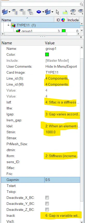
Defining parameter for Type 11 contact

• After defining the Type11 parameters, also with that we have to define the slave and master for Type 11 contact (Line id (S), Line id (M)
• Here also we need to request the TH/INTER which carry interface information in Time History file.
• Now we can run the simulation, for that go to Analysis panel >> RADIOSS >> select the input file >> save it in different folder and name it >> Run, also setting the -nt 3, whereas nt is number of threads or number of cores used to solve the problem.

• After completing the simulation, the RADIOSS will pop-up a solver window stating RADIOSS job completed, which indicates simulation has been finished, also showing the total number of cycle and Elapsed time, means time required to solve the problem.

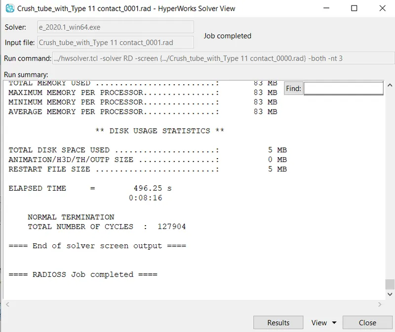
Total number of cycles = 127904

Elapsed time or computation time = 496.25

• Here as you notice that by introducing Type11 contact the computation time will increase.
• After running simulation animation files will be generated where we specified a location to store the file

To check the value of Energy error and Mass error, open the 0001.out file in Note pad

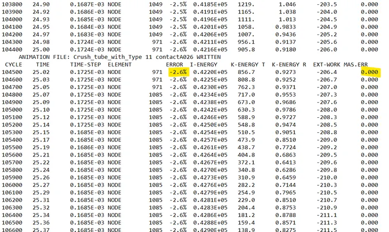
Here mass error is 0 and Energy error is -2.6%

• Here by introducing Type11 contact, energy error is decreased as compared to previous case.

• After that we need to visualize it. For that we need to switch to the Hyper-view utility, in hyper-view we need to import the h3d file that was generated during solving. Now to display the result we need to select the result plot we required, here we check von-misses contour by selecting Global variable as Von-misses, and here we use averaging method as simple to visualize the result.

• To plot the graph, we need to switch to the Hypergraph 2D. we can switch to it using the same client selector option in toolbar, also in single window we can split it into number of windows, where we can plot the different plots. To plot the graph, we required the T01 file to upload to see the graphs. This file is available in same directory where we have .out files, h3d files, here we can plot different graphs like Rigid wall forces, Internal energy, Kinetic energy, Hourglass energy, Total energy to compare and visualize the result.

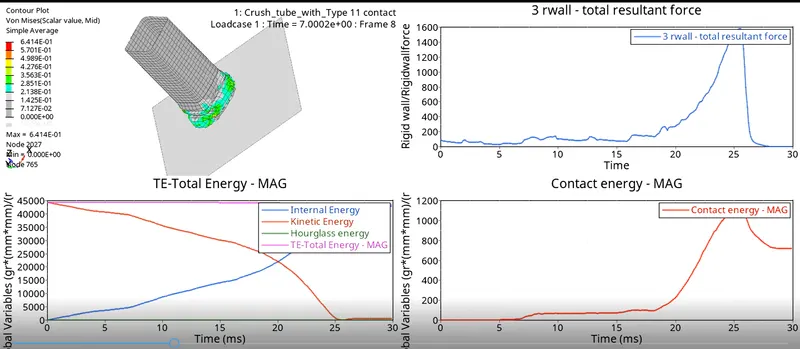
Rigid-wall force / Total energy / Internal energy / Kinetic energy / Hourglass energy / Contact energy

• Here in this case the Rigid wall force slightly increase as compared to previous case, because of adding type 11 contact, it also taken into account edge to edge contact, so due to this it avoids edge to edge penetration and leads to behave more stiff, due to this reaction forces which is nothing but rigid-wall forces, also the von-misses stress value decrease to some value as compared to previous case.
• But in this case, there is decrease in contact energy due to addition of type 11 contact, because it also taken into account edge to edge contact, so here penetration chances are less. Contact energy is the energy acting opposite to the system to prevent the penetration acting on the system. When the force is applied to the Body the crush tube starts to deform but the penetration happening low in the beginning, so due to this contact energy is low at initial stage. When deformation increases the penetration start increasing and large contact force is required to avoid penetration, here in this case along with Type 7, Type 11 contact is also defined that take care about edge to edge penetration, and this leads to decrease in the contact forces.

In case of edge is crossing or edge to edge contact take place TYPE11 interface can be added to capture the physics correctly.

Case 4: Remove both notches and remove Boundary condition on rigid body node and then run:

• Here in this case firstly we have to remove the notches and then we have to deleting the boundary condition of rigid body.

• To remove the notches, we can use Align option which is available in node edit Panel.

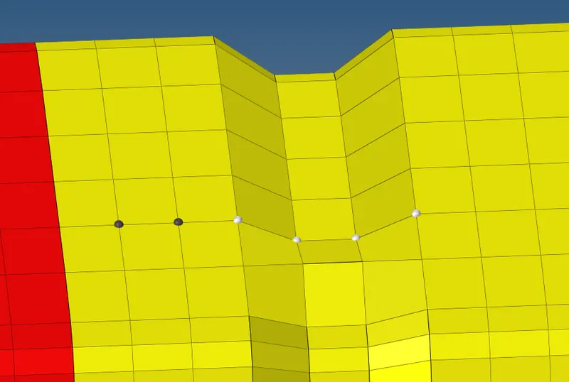
Using Align node option to remove the notches

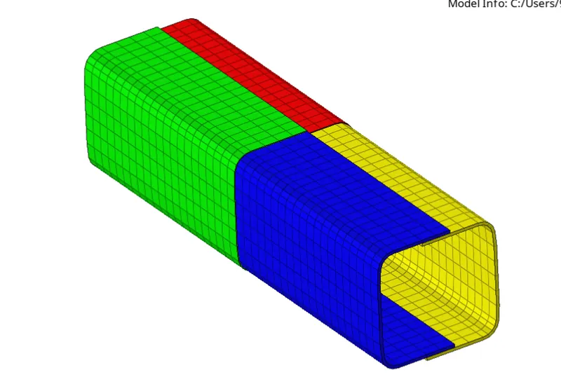
Notch Free Crush Tube

• After removing the notch, now we have to remove the Boundary condition of the rigid body nodes, for that go to Solver Browser >> Boundary condition, and delete the boundary condition.
• After removing the notches and deleting the boundary condition of rigid body nodes, now we can start solving the problem by using solver

• After completing the simulation, the RADIOSS will pop-up a solver window stating RADIOSS job completed, which indicates simulation has been finished, also showing the total number of cycle and Elapsed time, means time required to solve the problem.

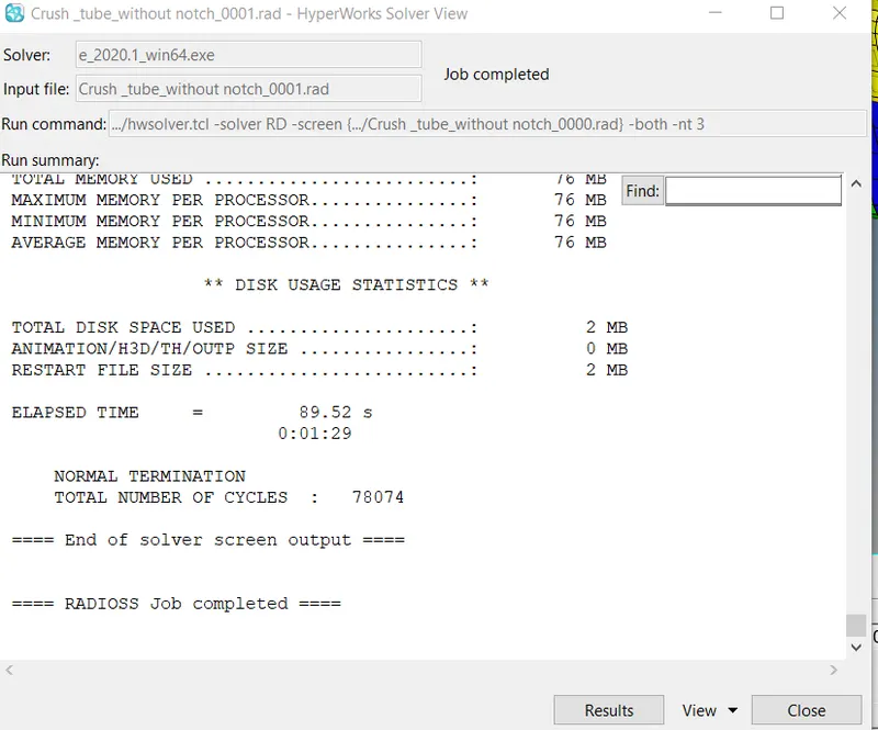
Total Number of cycles = 78704

Elapsed Time or Computation time = 89.52s

To check the value of Energy error and Mass error, open the 0001.out file in Note pad

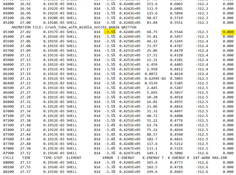
Energy Error and Mass Error

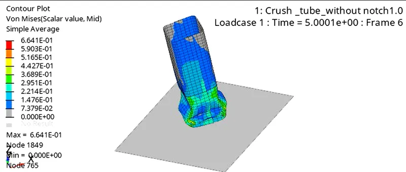
• After that we need to visualize it. For that we need to switch to the Hyper-view utility, in hyper-view we need to import the h3d file that was generated during solving. Now to display the result we need to select the result plot we required, here we check von-misses contour by selecting Global variable as Von-misses, and here we use averaging method as simple to visualize the result.

• To plot the graph, we need to switch to the Hypergraph 2D. we can switch to it using the same client selector option in toolbar, also in single window we can split it into number of windows, where we can plot the different plots. To plot the graph, we required the T01 file to upload to see the graphs. This file is available in same directory where we have .out files, h3d files, here we can plot different graphs like Rigid wall forces, Internal energy, Kinetic energy, Hourglass energy, Total energy to compare and visualize the result.

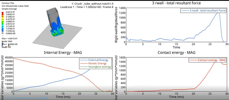
Rigid-wall force / Contact energy / Internal energy / kinetic energy / Hourglass energy

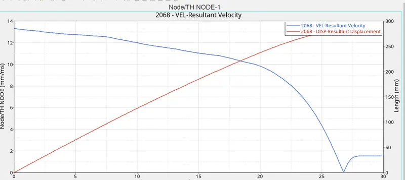
Resultant velocity vs Resultant Displacement

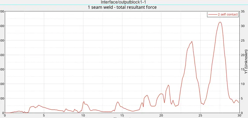
Self-Contact Force

• Here in this case, there is no notch present in the crash tube, due to this the bends in tube or crushing of tube star from the bottom portion where it strikes the wall, and bends start increasing with time due to this there is rise and fall in the Rigid wall forces. After the deformation was complete the graph decreases suddenly and got a constant value after th e deformation. The total resultant force value is 1350N
• Similarly kinetic energy decreases with time and internal energy increases due to bends in tube that absorb the energy due to this there is rise in the Internal energy with deformation.
• Here in this case Contact energy and contact forces are decreases due to absence on notches. Because we know that contact energy is energy acting opposite to the system to prevent penetration acting on the system, when the force is applied to the body the crush tube starts to deform, but the penetration happening is low at the initial stage, so the contact energy will low at initial state. With time rate of deformation start increasing the element will forced to penetrate but the opposite force which is contact energy will also increase which helps in prevention of penetration, but here in this case due to absence of notches deformation is not much high, due to this contact energy value is low, as compared to case1 and case 2

Case 5: Create a new notch in the middle, select the whole section and run

• In this case we are using the same file of case 4 (Crush tube without notches)
• To create the notches at middle we can use the translate option which is available in Tool panel.

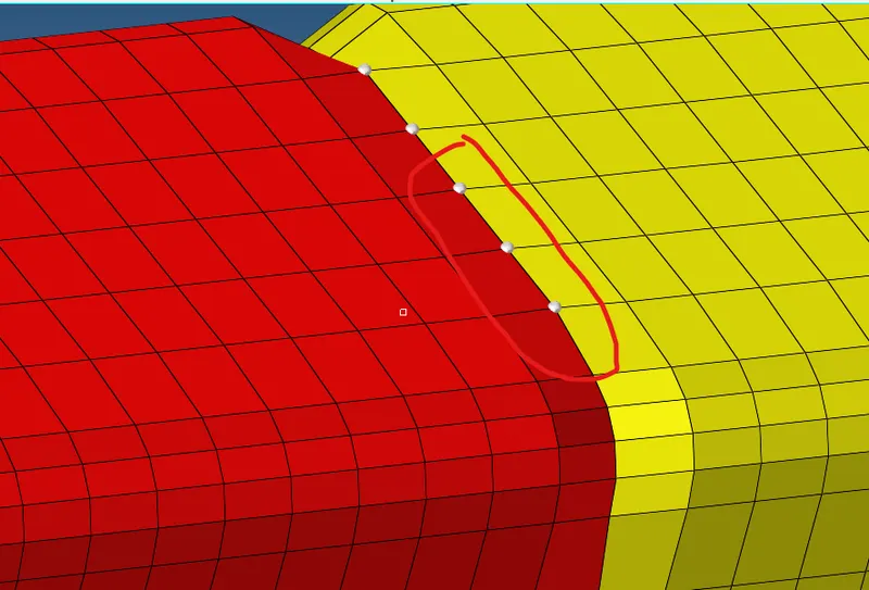
Translate node to creates the notches

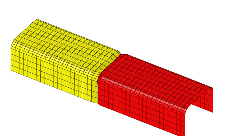
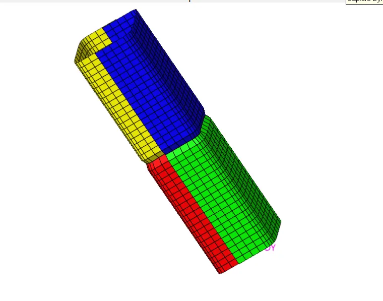
Notch created at middle od crush Tubes

• Now after creating the notch, we can start to solve the file by using solver

• After completing the simulation, the RADIOSS will pop-up a solver window stating RADIOSS job completed, which indicates simulation has been finished, also showing the total number of cycle and Elapsed time, means time required to solve the problem.

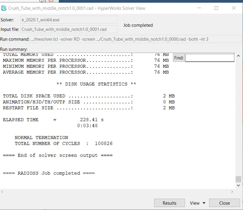
Total number of cycles = 100826

Elapsed time or Computation time = 228.41s

To check the value of Energy error and Mass error, open the 0001.out file in Note pad

Here the mass error is 0 whereas the energy error is -3.5% which is under acceptable range

• After that we need to visualize it. For that we need to switch to the Hyper-view utility, in hyper-view we need to import the h3d file that was generated during solving. Now to display the result we need to select the result plot we required, here we check von-misses contour by selecting Global variable as Von-misses, and here we use averaging method as simple to visualize the result.

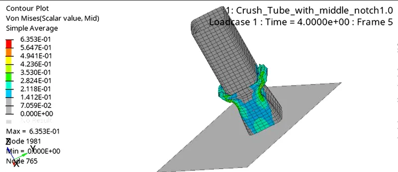
Von-Misses plot

• To plot the graph, we need to switch to the Hypergraph 2D. we can switch to it using the same client selector option in toolbar, also in single window we can split it into number of windows, where we can plot the different plots. To plot the graph, we required the T01 file to upload to see the graphs. This file is available in same directory where we have .out files, h3d files, here we can plot different graphs like Rigid wall forces, Internal energy, Kinetic energy, Hourglass energy, Total energy to compare and visualize the result.

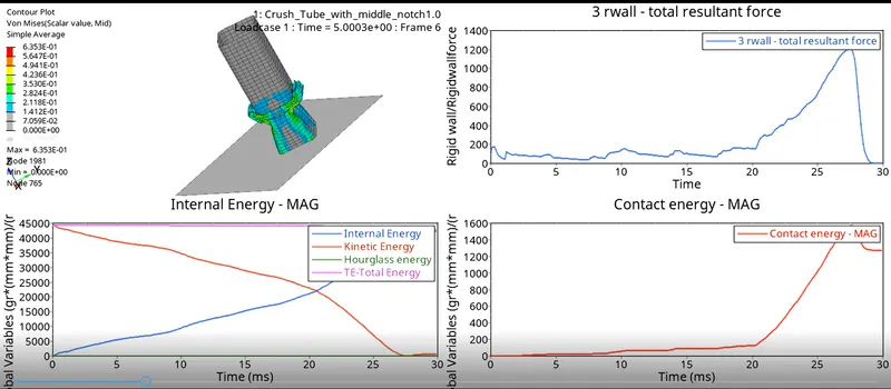
Rigid-wall force / Contact energy / Internal energy / kinetic energy / Hourglass energy

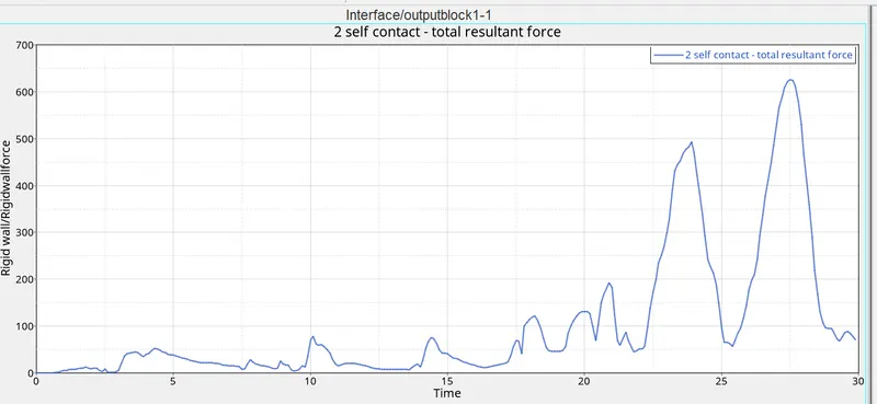
Self-contact force

• Here in this case the contact energy is increasing as compared to previous case (without notch case), Here in this case there is notch present at the middle due to this there is increase in the rate of deformation which intern increase the rate of penetration, as penetration increases then force required to remove penetration which is nothing but the contact energy is also increases.

Case 7: Create a new notch with nodes only from opposing two face and run

• Here we again import the 0000.rad file of case4 where there is no notch present at the crush tube.

• Now to create the notches at middle again we use the translate option to create the notch, by moving the nodes inward normal to the surface.

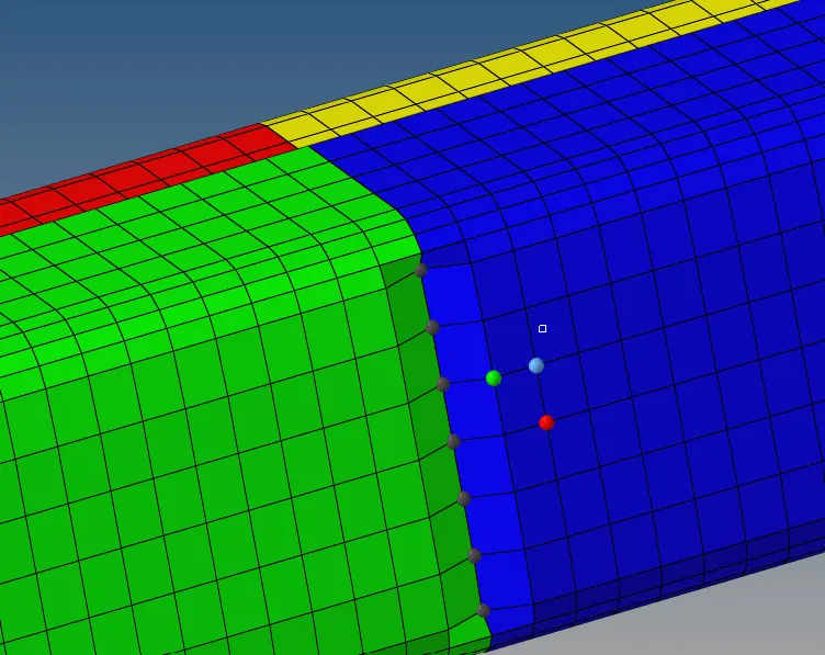
Creating a Notch by using translate option

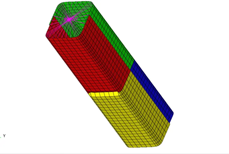
Notch is created at both two opposite Faces

• Here also we need to create the TH/INTER which is nothing but Total contact energy in the global parameter.

• After that now we can start to solve the problem by using solver for that go to Analysis >> RADIOSS, define the file and save it and also define the number of threads or number of cores to be used, after that click on RADIOSS to run the simulation.

• After completing the simulation, the RADIOSS will pop-up a solver window stating RADIOSS job completed, which indicates simulation has been finished, also showing the total number of cycle and Elapsed time, means time required to solve the problem.

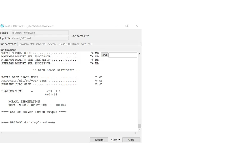
End of solver screen output

To check the value of Energy error and Mass error, open the 0001.out file in Note pad

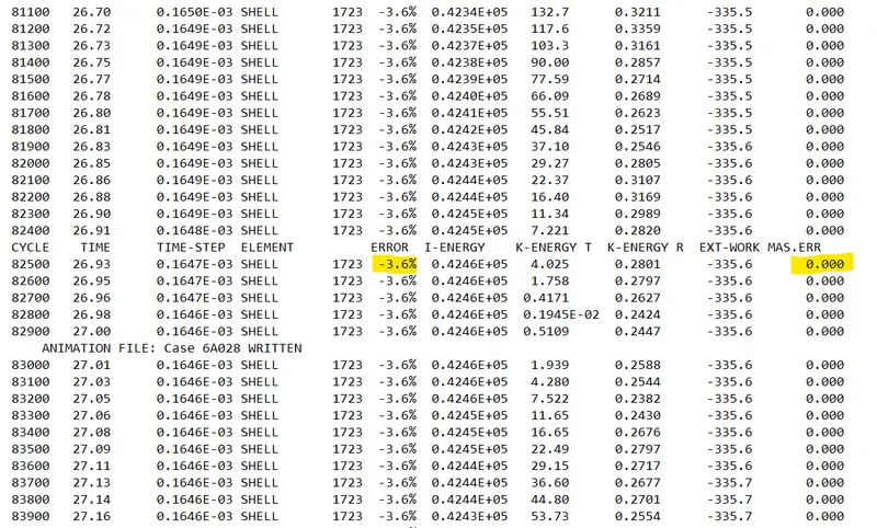
Here the mass error is 0 but the energy error is -3.6% which is under acceptable range

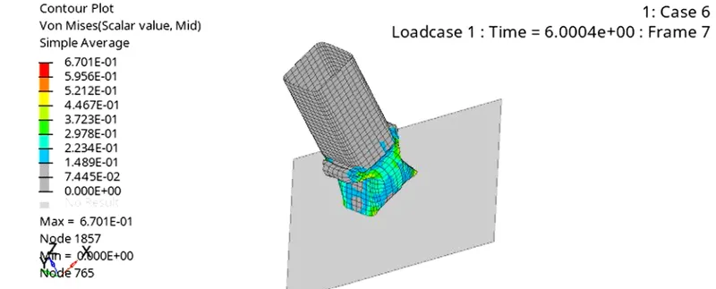
• After that we need to visualize it. For that we need to switch to the Hyper-view utility, in hyper-view we need to import the h3d file that was generated during solving. Now to display the result we need to select the result plot we required, here we check von-misses contour by selecting Global variable as Von-misses, and here we use averaging method as simple to visualize the result.

• To plot the graph, we need to switch to the Hypergraph 2D. we can switch to it using the same client selector option in toolbar, also in single window we can split it into number of windows, where we can plot the different plots. To plot the graph, we required the T01 file to upload to see the graphs. This file is available in same directory where we have .out files, h3d files, here we can plot different graphs like Rigid wall forces, Internal energy, Kinetic energy, Hourglass energy, Total energy to compare and visualize the result.

Rigid-wall force / Contact energy / Internal energy / kinetic energy / Hourglass energy

Self-Contact Force

• Here also in this case, the bend will first start at the notch section, due to this bend rigid-wall forces decline and due to continuous deformation rigid wall forces decreasing with time, after 15 ms there is again rise in the graph because, now there is not enough material to deform, the reaction forces increase as shown in figure, it is increases up to some value and then decline, because there is no more force present that push that crush tube.

• Here in this case also the contact energy is increased, again due to notch present at the middle there is increase in the rate of deformation which intern increase the rate of penetration, as penetration increases then force required to remove penetration which is nothing but the contact energy is also increases.

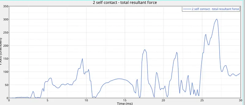
• Here as you see there is lot of fluctuation in self contact force, which is nothing but the force transmitted by the contact, those fluctuation is basically due to bends or we can say crumple occurring in crush tube with time.

Conclusion / Learning outcomes:

• From all the cases we can say that “Inacti” is required to be defined if we use the Type 7 contact, because it is very sensitive to initial penetration. So Inacti flag will help us to remove the initial penetration if they exist in the model.
• For crash and Impact analysis we generally used TYPE7 contact which is basically node to surface contact, but for more complex cases like air bag folding simulations we can use type7 along with type 11 which basically is edge to edge contact, but we have to use type11 with precautions because it increases the computational cost.
• So crash tube or crash box is like tube shape object which is located between bumper and chassis, these will help to reduce impacts energy during collision, during impact shock energy is converted into strain energy or internal energy by crumpling of crash box or crash tube. So crash box or tube require reduced buckling mode, so that instead of bending it should crumple and absorb large amount of energy. One important observation from these simulations is that by introducing notch, the tube will crumble from the notch region first, so from here it is clear that by introducing notch, our tube got easily crumpled and start absorbing the large amount of energy.