Assignment 5-RADIOSS Interfaces & Study of Effect of Notches Challenge

 Aim-

• Perform 2D mesh on bumper assemblygiven with 6mm element size.
• Run the crash tube model with diffrenet types of interface contacts.

Objective-

• Run the crash tube model as it given.
• Change the inacti-6 to avoid initial penetration and run the model.
• Create type 11 type contact with required parameter.
• Removing of notch over the crash tube and boundary conditions on rigid body node and run.
• Create new notch at in middle and run the model.
• Create new notch on opposite faces only ad run the model.
• Postprocessing of all cases,review the model in hyperview and graphs in hypergraph 2D.

Procedure-

1. clean the geometry on which we are going to mesh.

a).

• Here use surface intersection to join both surface.
• Go to surface edit > trim with surface plane > self intersecting surface.

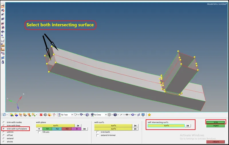
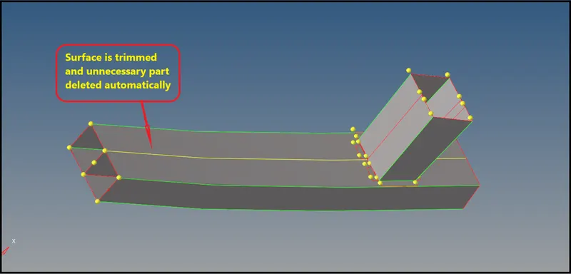
b).

•  Now perform equivalence on overlaping surfaces, with 10mm search distance.

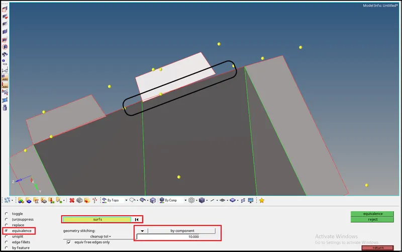
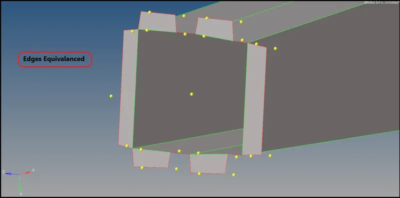
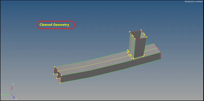
• Geometry cleanup is done.
• Once cleanup is done go for meshing,

 Go to 2D > automesh > select surface > mesh size-6mm

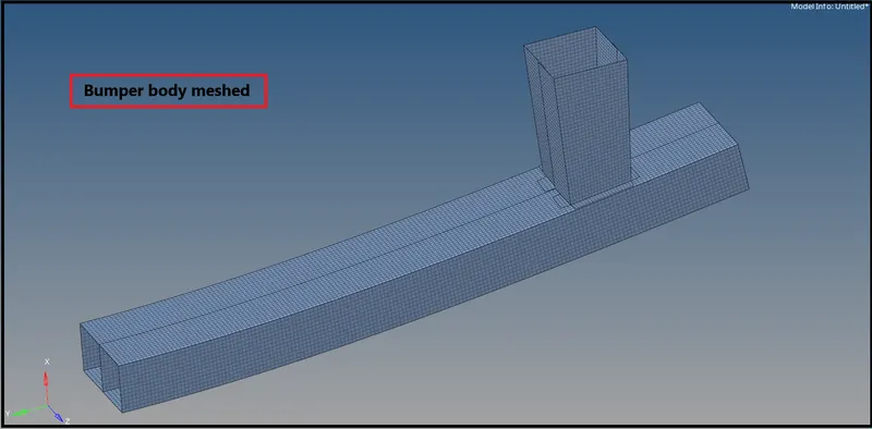
2).

Import the starter file in radioss solver deck.

 

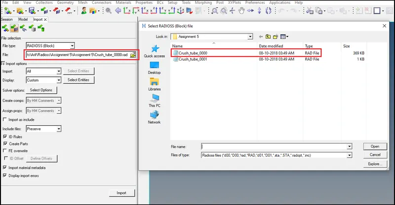
• Select appropriate starter file of crash tube and type of file as radioss files.
• Now open the file in hypermesh GUI.

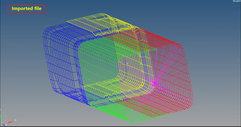
• Above representation is in wireframe mode.
• Now turn on shaded mode for proper representation of elements.

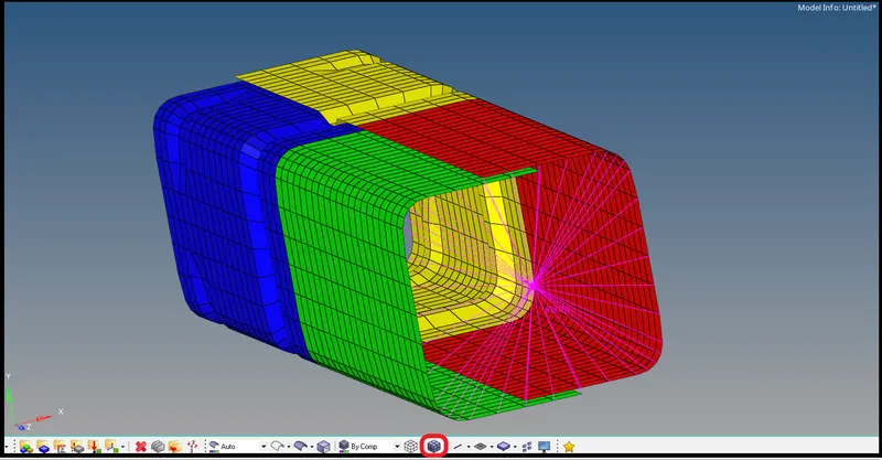
Case-1:Run the simulation as it given.

Now run the simulation-

• To run the simulation go to Analysis > Radioss.

• After clicking Radioss click on input file and save it in new folder as Case-1.
• Check the include connectors and option as -nt 4.
• N indicated the how many cores will involve to run the simulation.
• It will make simulation faster. 

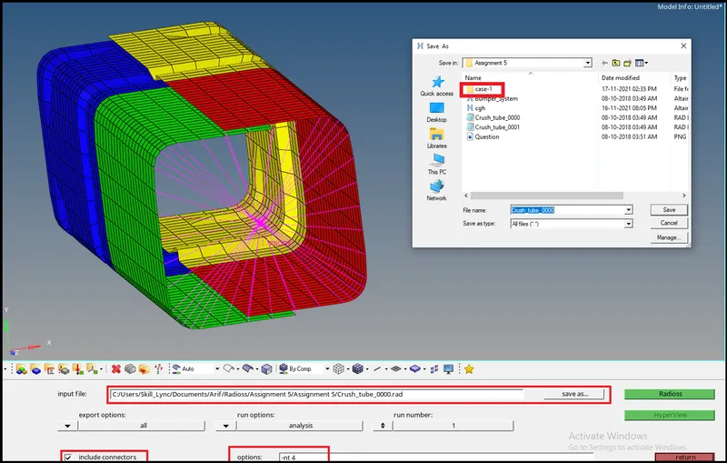
• After that click on Radioss it will start the simulation.
• And wait untill the new window popup and show as Radioss job completed.
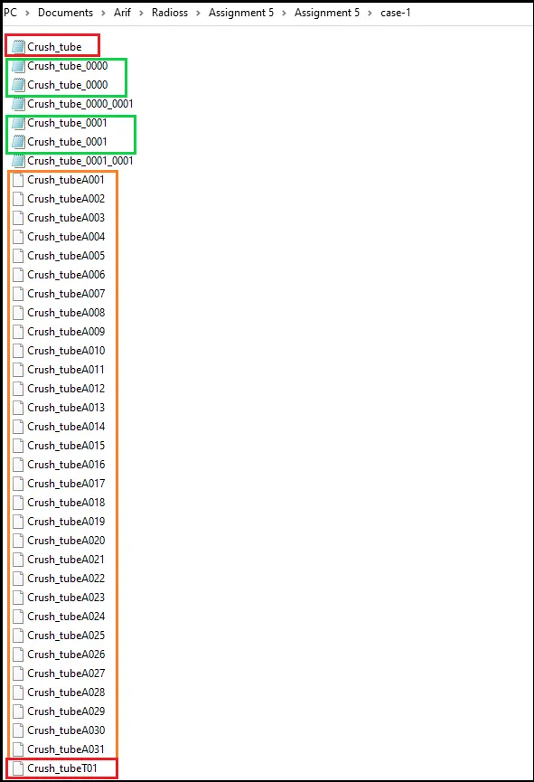
• Now after running the simulation we got animation file also.
• Now run the simulation and save the radioss file as different case as case-1.
• After running the simulation we will get animation file, h3d file and also T01 file.

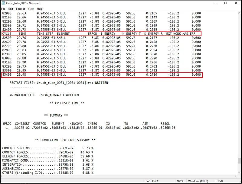
• Now open 0001.out file and check all the details. 
• Here we can see all variable in the out file about energy and mass loss also.
• So for checking the maximum loss check the last cycle details.

Post processing-

• Review the simulation using Hyperview.
• Plot the graphs using Hypergraph-2D

1.Review the simulation using Hyperview.

Split the screen in two part-

 

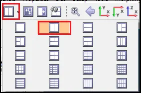
• Now after splitting the sreen open hyperview after switching into in 2nd screen.

• In hypergraph window import the h3d file for simulation run.

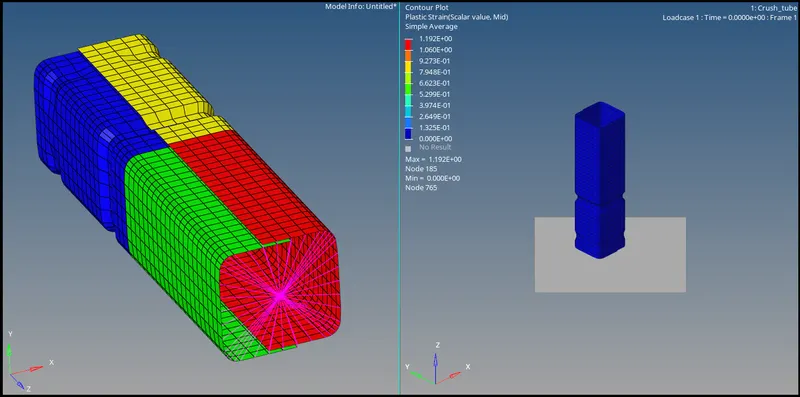
• Now after importing the h3d file on hyperview GUI go for contour activation.
• In contour it will show the simulation graphically and contour lies of load and other properties variation.
• To activate contour go to Tool bar > contour as shown below.
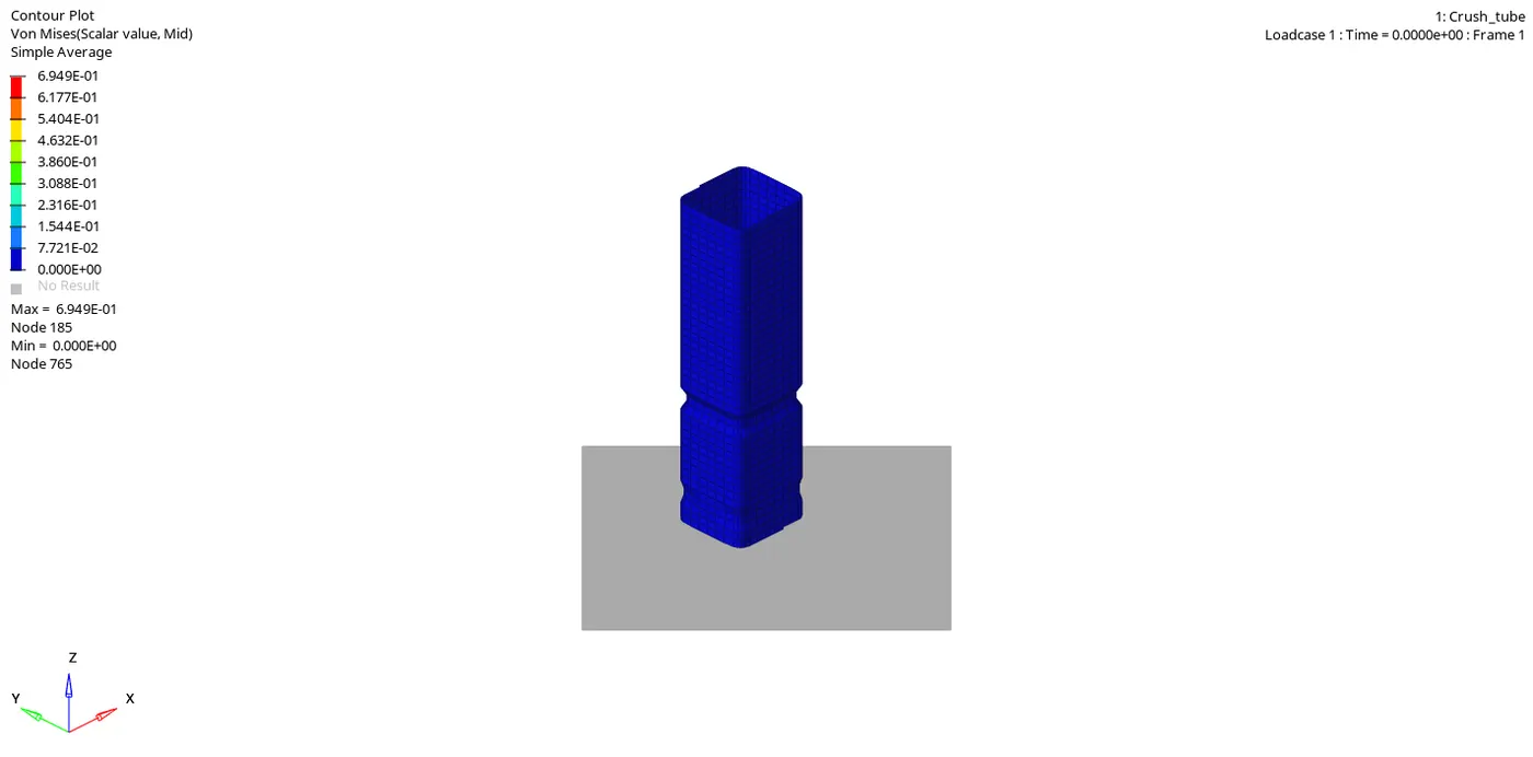
• Go to Contour > von-mises > averaging methode as simple > apply contour.

• simillarly for plastic strain-

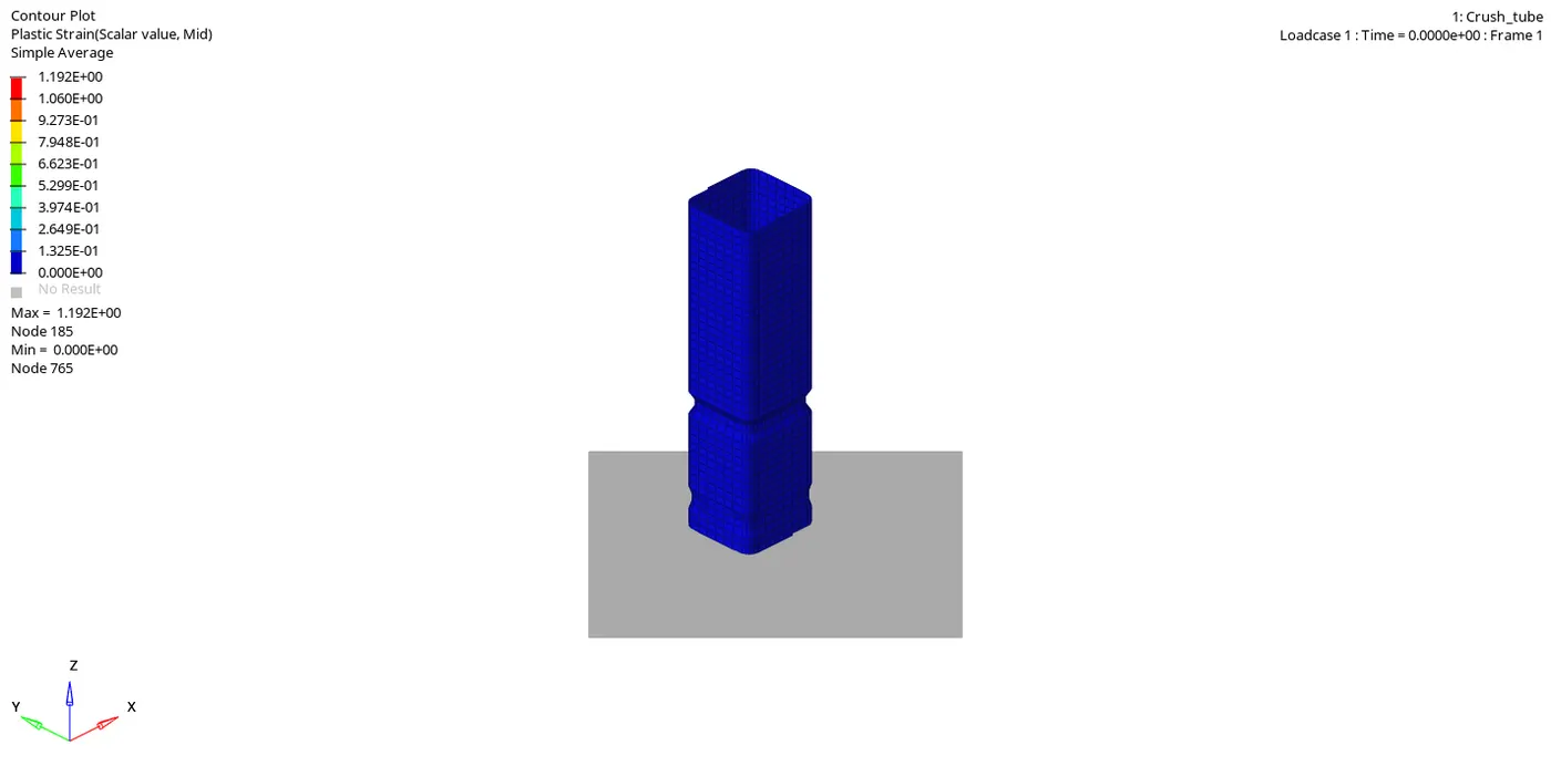
• In above hyperview values we can see that the tube start bending on notches.It starts from first notch and then second notch bend.
• And region between two notches is getting crashed.
• And finally the region above middle notch then crashed,
• So we will found that the maximum von mises stress and maximum plastic strain value will be found on throughout the corner of tubes as we can see in above animation.

 2. Plot the graphs using Hypergraph-2D

• Now split the window in 3Part and open hypergraph-2D in new window.
• After opening the hypergraph window import the T01 file in Hypergraph.

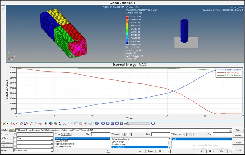
Go to Global Energy > Kinetic energy+Internal Energy+Total energy > Magnitude > solver unit > apply.

Global Energy graphs-

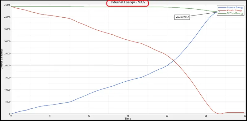
• Initially we can see that kinetic energy is maximun since tube is crushing and elements are moving.
• Initially elements are moving with faster rate and by time passes deformation is also taking place so that energy will strat converting into internal energy.
• So thats why kinetic energy and internal energy graphs are cross proportional to each other in this case.
• And total energy will be constant since its combination of energies, yes there is some drop in total energy graph because of loss of energy in  friction occuring between the elements.

Rigid wall force-

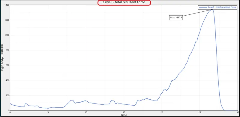
• Rigid wall force apllied by rigid plate to tube, initially crushing starts from bottom side of the tube at that moment slave nodes of tube try to penetrate into rigid plate master segment at that point spring stiffness increses force try to oppose the salve node thats why we can se little increment in graph with respect to time till 20th ms.
• Till 20th ms whole tube crushed about 80-90%(gif below), at that point lot of slave nodes came near master segment.

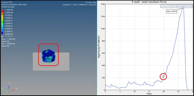
• So from that particular point nedd more force to appose the slave node due to that graph is increasing suddenly.
• Force drop to zero after complete crush.

Contact energy-

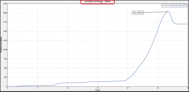
• Initially we can see contact graph is at lower because initially deformation is less and contact between tub elements are less.
• As tube getting crushed 80-90% mainly after 20th ms most of the elements are in contact closely so at that point contact energy will boom to higher value.
• This contact force is actually helps to craete spring force which result to avoid penetration between elements.
• The graph is decreasing after some time just because of after complete crush of tube it rebound back of some portion so contact forces will decrease.

Case-2  :Change the Inacti=6 an run the model.

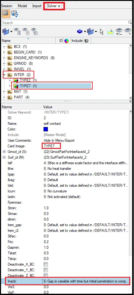
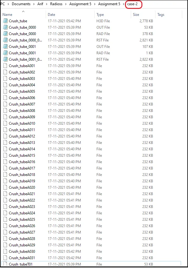
•  Now run the simulation and save the radioss file as different case as case-2.
• After running the simulation we will get animation file, h3d file and also T01 file.

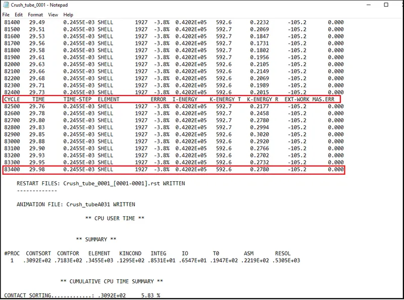
• Now open 0001.out file and check all the details. 
• Here we can see all variable in the out file about energy and mass loss also.
• So for checking the maximum loss check the last cycle details.

 

Post processing-

• Review the simulation using Hyperview.
• Plot the graphs using Hypergraph-2D

1.Review the simulation using Hyperview.

• Now after importing the h3d file on hyperview GUI go for contour activation.
• In contour it will show the simulation graphically and contour lies of load and other properties variation.
• To activate contour go to Tool bar > contour as shown below.
• Go to Contour > von-mises > averaging methode as simple > apply contour.

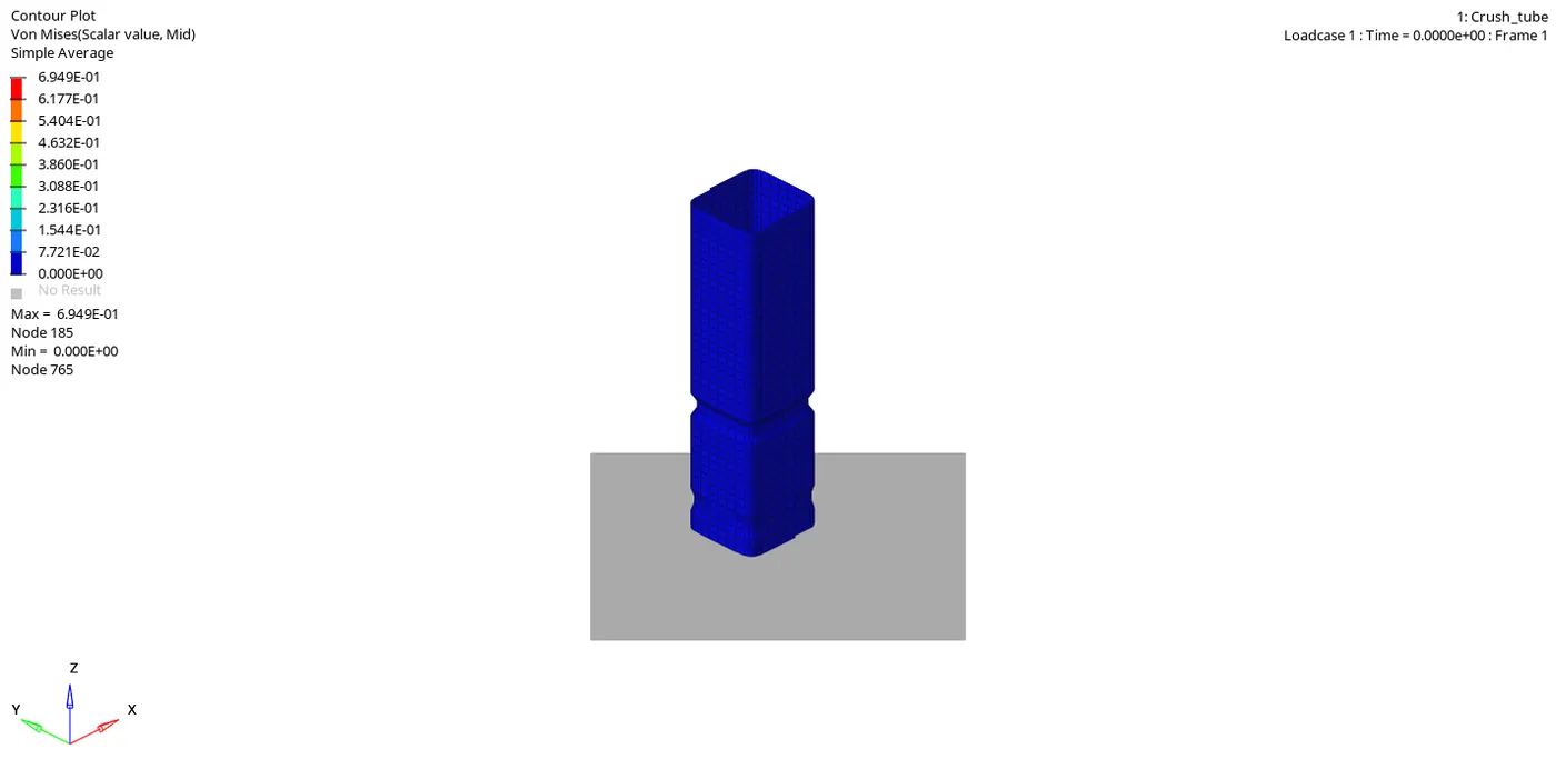
• simillarly for plastic strain-

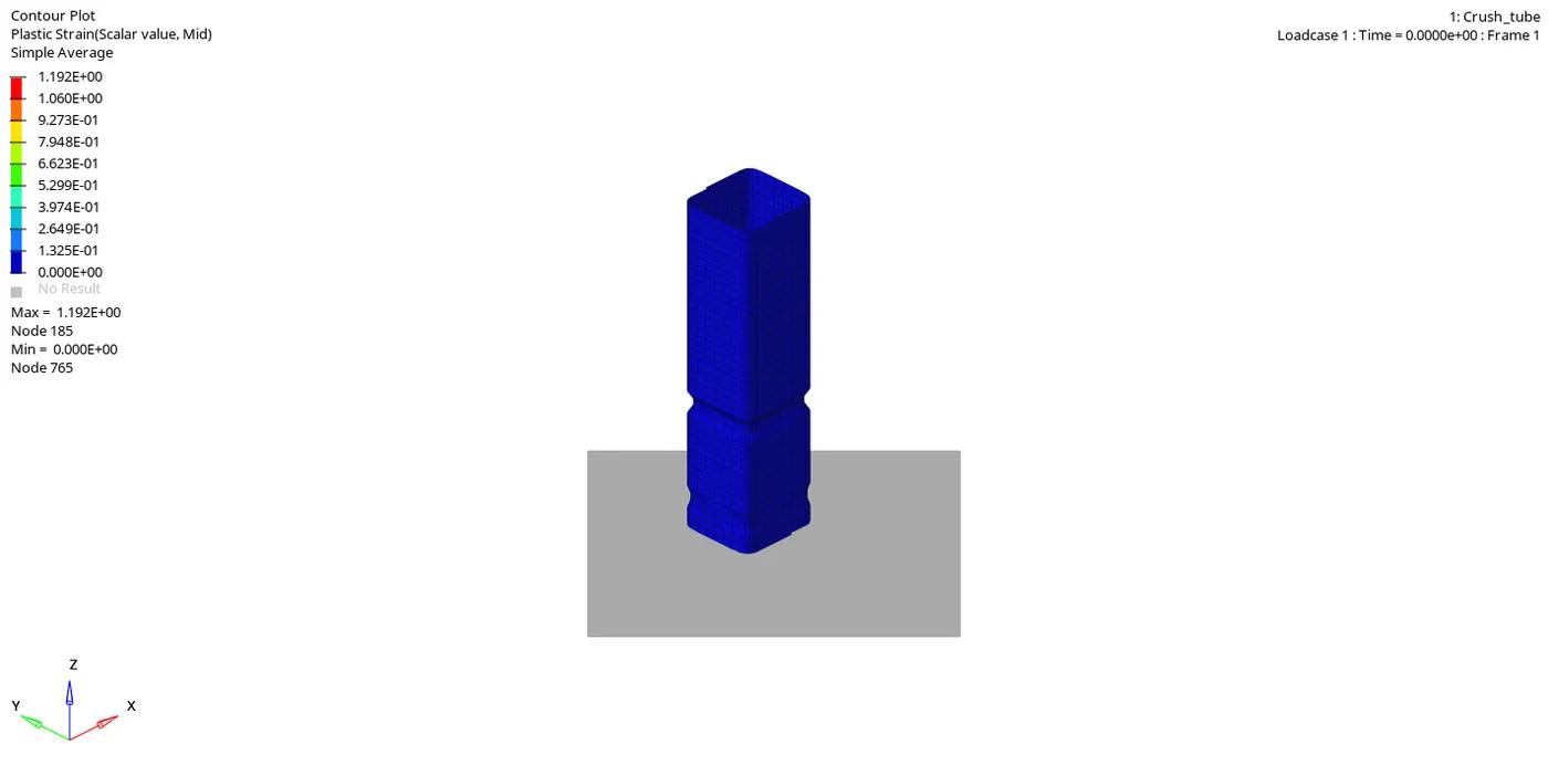
• In this case also we will find same behaviour of simualtion as case-1 cause here have only change Inacti=6 which helps in initial penetration.
• What Inacti do is it will move the salve node to 30% of initial penetration happening in the simulation to avoid contact stability issue.
• Since we activated Inacti=6 before simulation thats why we are not able to se any difference in simulation.

2. Plot the graphs using Hypergraph-2D

• Now split the window in 3Part and open hypergraph-2D in new window.
• After opening the hypergraph window import the T01 file in Hypergraph.

Go to Global Energy > Kinetic energy+Internal Energy+Total energy > Magnitude > solver unit > apply.

Global Energy graphs-

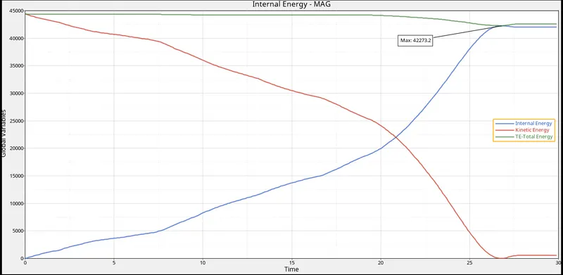
• The energy graphs we will see same as case-1.

Rigid wall force-

• Here in this case also elements going into contact with rigid wall same as case-1 so nehaviour of curve will also be same as 1st case.

Contact energy-

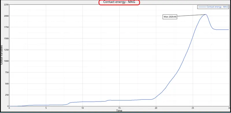
• In this case also contact energy will increase in order to elemental contact with respect to time.

Case-3 : Create the type 11 contact and run.

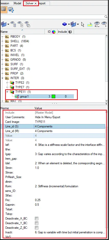
To create Go to solver> INTER> Create >Type11>Set all the recomended parameter

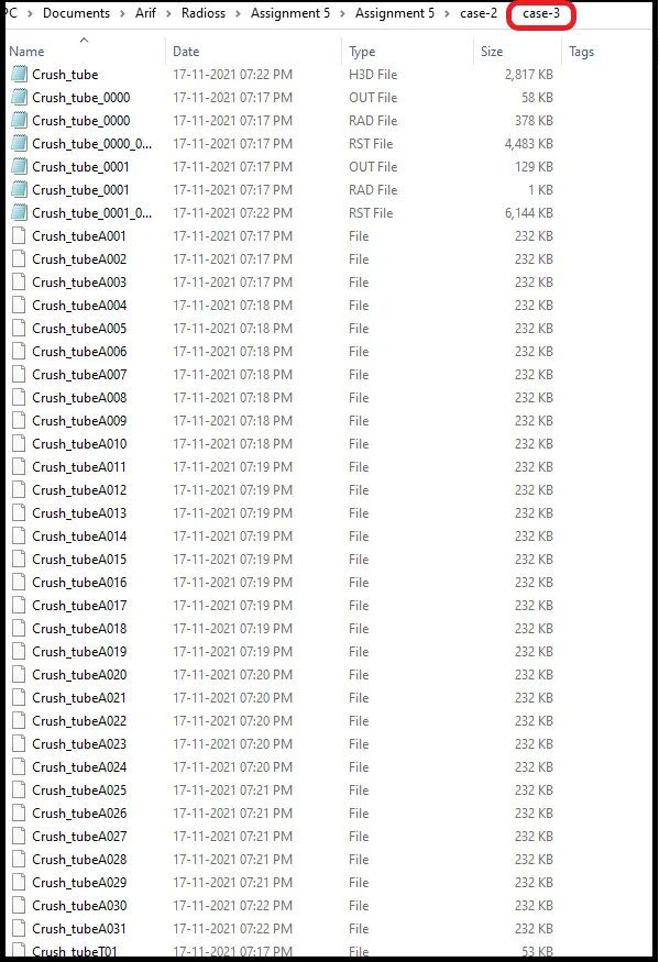
•  Now run the simulation and save the radioss file as different case as case-3.
• After running the simulation we will get animation file, h3d file and also T01 file.

 

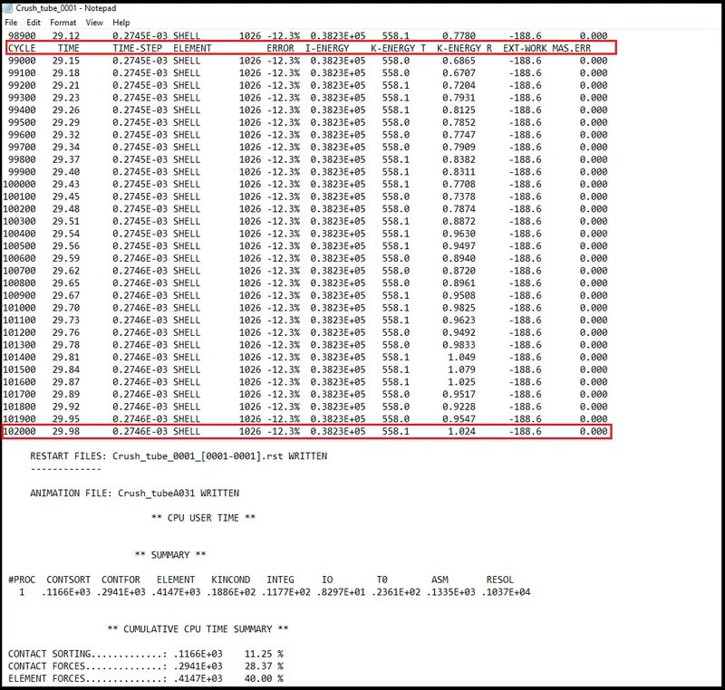
• Now open 0001.out file and check all the details. 
• Here we can see all variable in the out file about energy and mass loss also.
• So for checking the maximum loss check the last cycle details.

Post processing-

• Review the simulation using Hyperview.
• Plot the graphs using Hypergraph-2D

1.Review the simulation using Hyperview.

• Now after importing the h3d file on hyperview GUI go for contour activation.
• In contour it will show the simulation graphically and contour lies of load and other properties variation.
• To activate contour go to Tool bar > contour as shown below.
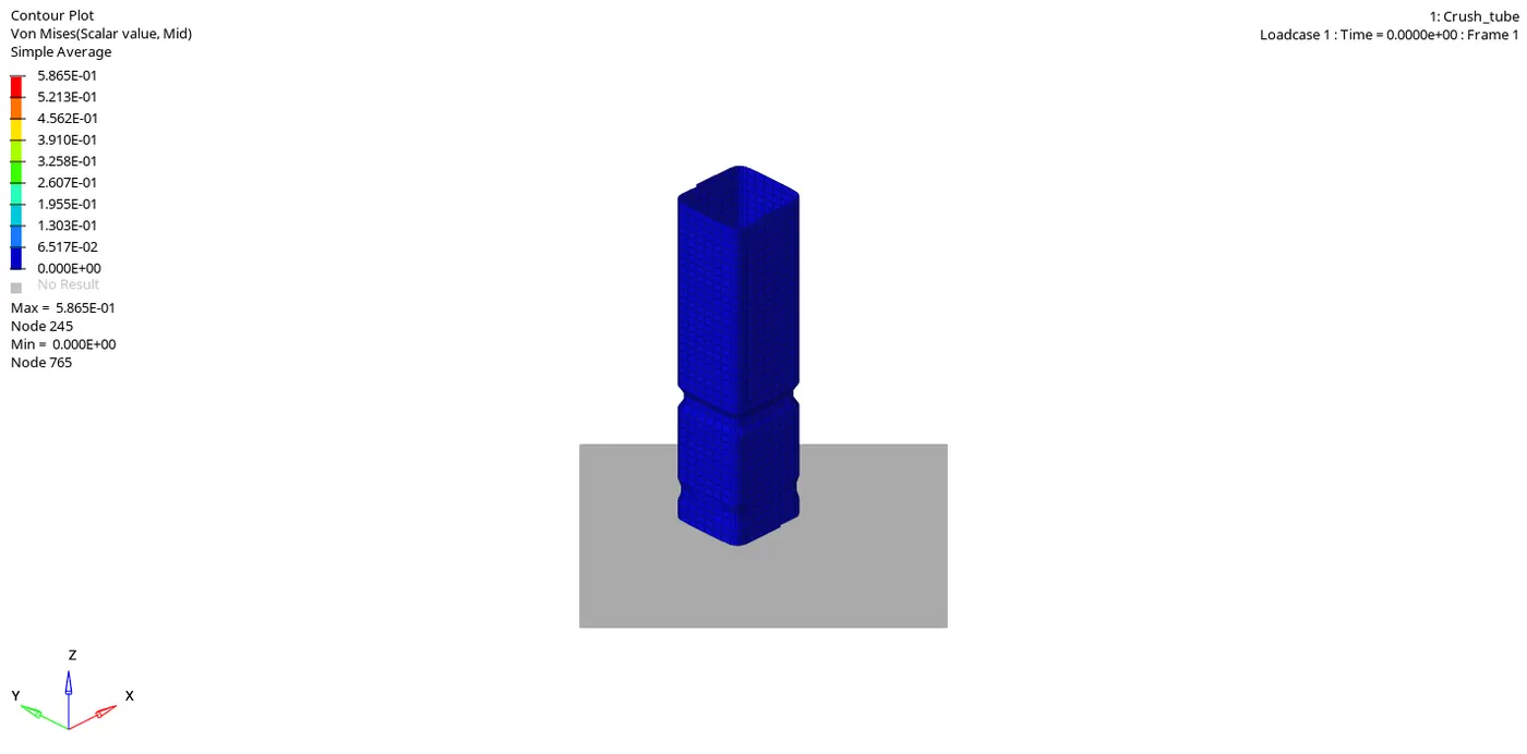
• Go to Contour > von-mises > averaging methode as simple > apply contour.

• simillarly for plastic strain-

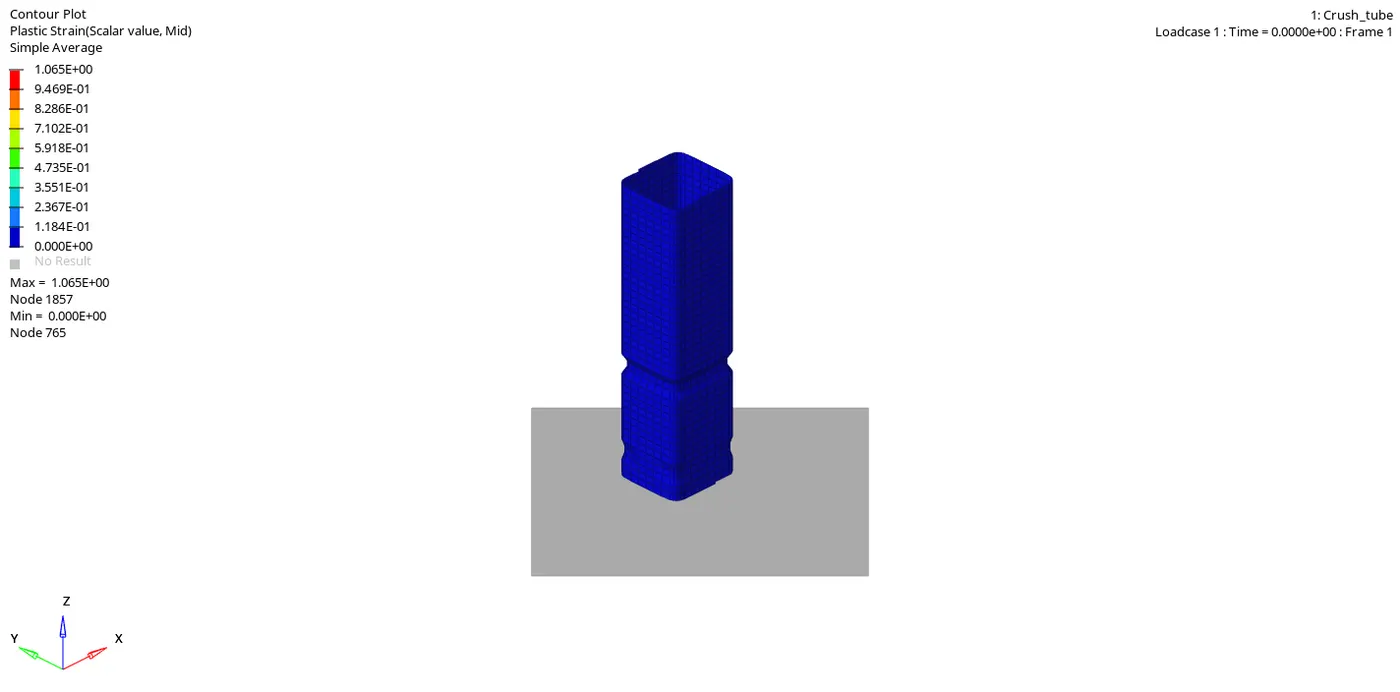
• In this case we used type 11 interfaces which helps in avoiding edge to edge interaction which we have seen in previous case.
• In this case we will notice little less von-mises stress and plastic strain value.Rest of the result will be approximate to previous case.

2. Plot the graphs using Hypergraph-2D

• Now split the window in 3Part and open hypergraph-2D in new window.
• After opening the hypergraph window import the T01 file in Hypergraph.

Go to Global Energy > Kinetic energy+Internal Energy+Total energy > Magnitude > solver unit > apply.

Global Energy graphs-

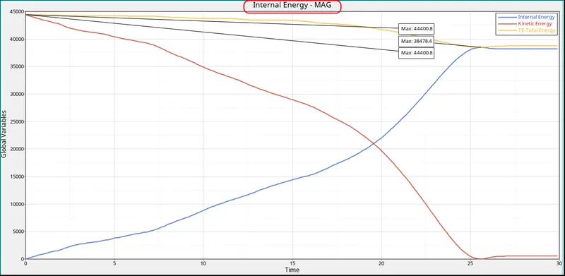
• In this case we can see little more drop in total energy and less gain in internal energy that is because of edge to edge interaction are not happeneing, so that deformation is also less in this case.
• So that gain in internal energy is less as compare to previous case.

Rigid wall force-

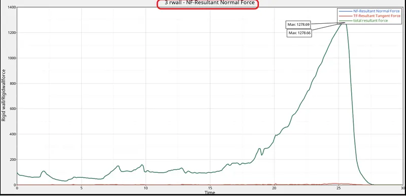
• In same manner due to less deformation the force acting by elements to rigid wall will be less.

Contact energy-

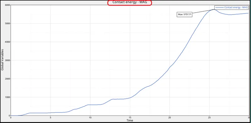
• In contact energy also due to less deformation no of elements getting into contact is also less.
• So there is little less gain in contact energy.

Case-4 :Remove both notches  and remove boundary condition on rigid body node then run.

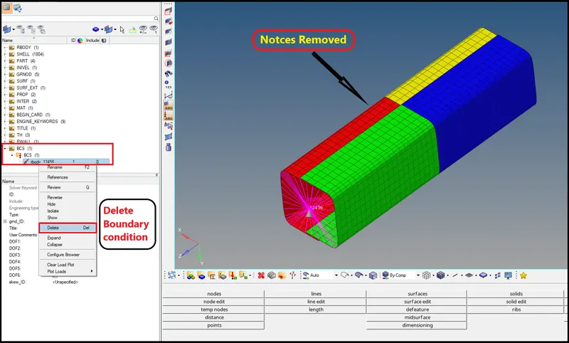
• To remove notches go to Edit node>Align node and select nodes to align.
• For deleting boundary condition go to solver > BCS > Delete boundary condition.

•  Now run the simulation and save the radioss file as different case as case-3.
• After running the simulation we will get animation file, h3d file and also T01 file.

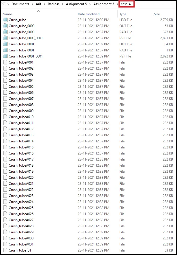
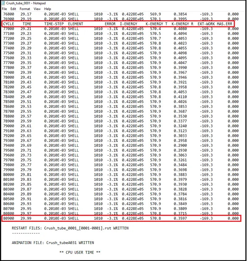
• Now open 0001.out file and check all the details. 
• Here we can see all variable in the out file about energy and mass loss also.
• So for checking the maximum loss check the last cycle details.

Post processing-

• Review the simulation using Hyperview.
• Plot the graphs using Hypergraph-2D

1.Review the simulation using Hyperview.

• Now after importing the h3d file on hyperview GUI go for contour activation.
• In contour it will show the simulation graphically and contour lies of load and other properties variation.
• To activate contour go to Tool bar > contour as shown below.
• Go to Contour > von-mises > averaging methode as simple > apply contour.

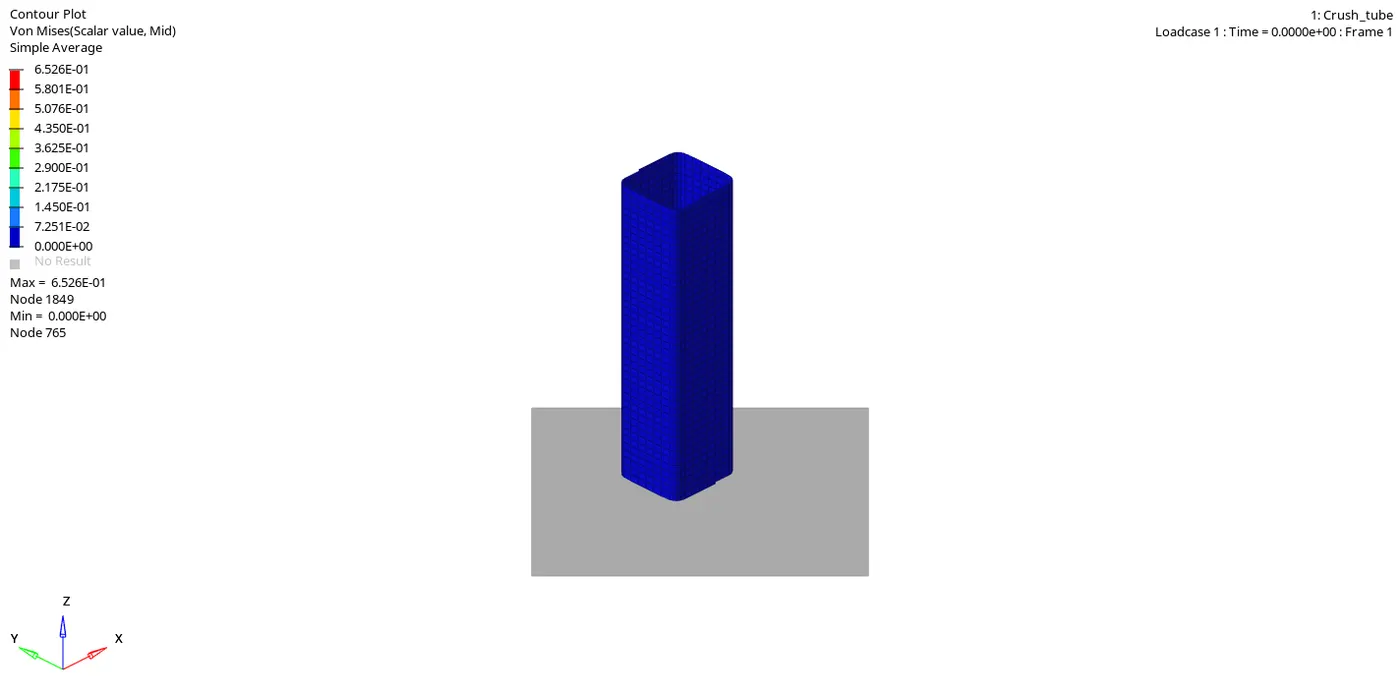
• simillarly for plastic strain-

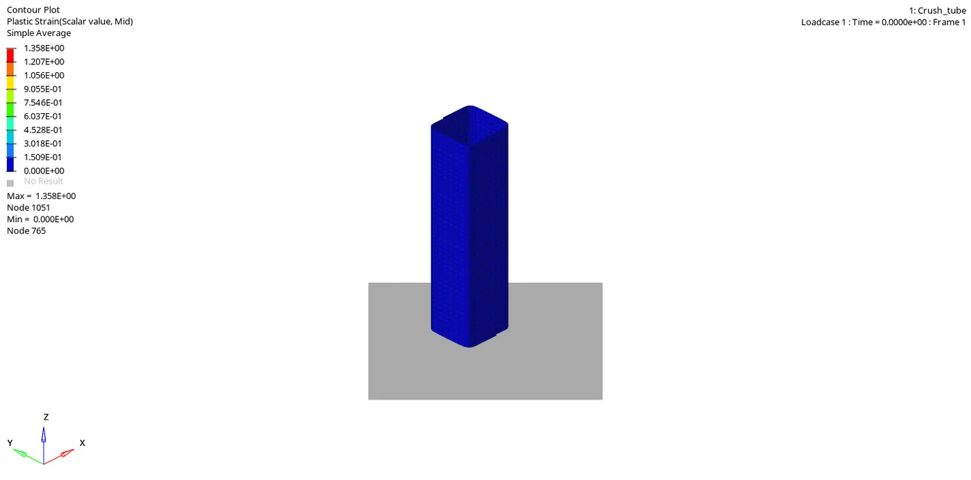
• In this case we have removed notch, so that the tube deformation will be uniform means there is no weak point for higher stress concentration.
• So the deformation will start from bottom end beacuse that end coming into contact with wall.In previous case also bottom end coming into contact but the moment after bottom edge gets into contact to wall the amount of stress found higher at notch area.thats why deformation start from notch area.
• So tube starts deforming from bottom edge in layered.Von-mises stress is also less in this case due to absence of notch.

2. Plot the graphs using Hypergraph-2D

• Now split the window in 3Part and open hypergraph-2D in new window.
• After opening the hypergraph window import the T01 file in Hypergraph.

Go to Global Energy > Kinetic energy+Internal Energy+Total energy > Magnitude > solver unit > apply.

Global Energy graphs-

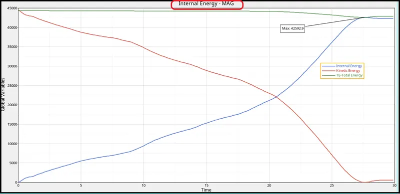
• In this case the total energy and internal energy graph variation is approx simmilar to 3rd case.

Rigid wall force-

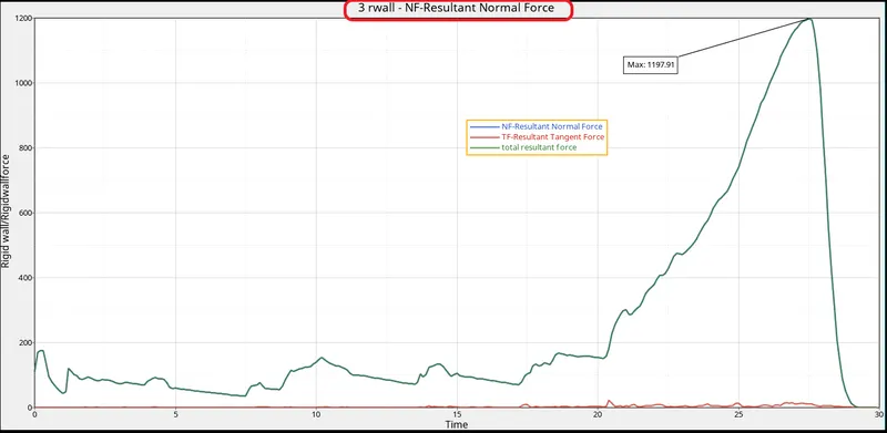
• The resultent rigid wall forces will decrease(Less than 1200KN) compared to previous case because here in this case we had removed boundary condition.

Contact energy-

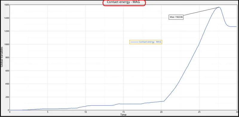
• Contact energy is also reduced compared to previous case is because of removal of notch and boundary condition.
• Due to removal of notches deformation is layered and uniform thats why contact between elements are less.

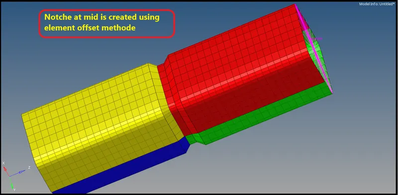
Case-5 :Create a new notch in the middle ,select the whole section and run.

•  Now run the simulation and save the radioss file as different case as case-5.
• After running the simulation we will get animation file, h3d file and also T01 file.

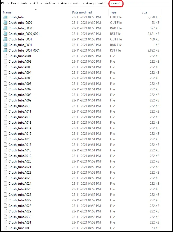
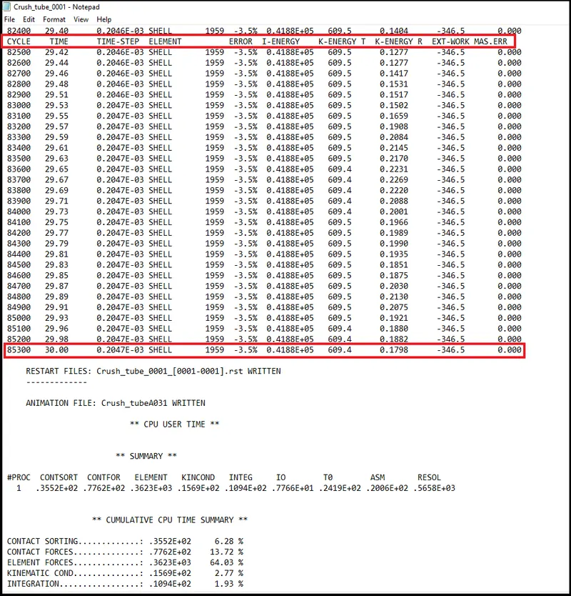
• Now open 0001.out file and check all the details. 
• Here we can see all variable in the out file about energy and mass loss also.
• So for checking the maximum loss check the last cycle details.

Post processing-

• Review the simulation using Hyperview.
• Plot the graphs using Hypergraph-2D

1.Review the simulation using Hyperview.

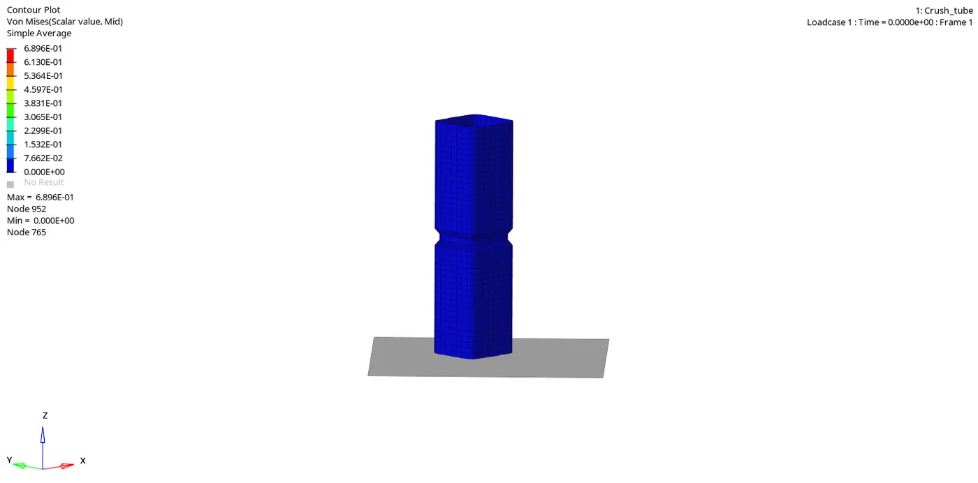
• Now after importing the h3d file on hyperview GUI go for contour activation.
• In contour it will show the simulation graphically and contour lies of load and other properties variation.
• To activate contour go to Tool bar > contour as shown below.
• Go to Contour > von-mises > averaging methode as simple > apply contour.

• simillarly for plastic strain-

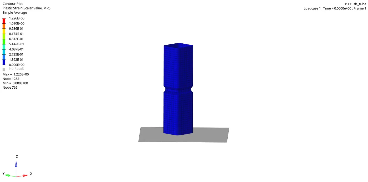
• Here in this case one notch is created at the mid so deformation will start from notch only due to higher stress concentration.
• Von-mises and plastic starin value is approximately simmilar to case-1.As in case-1 two types of notch was there.
• But here von-misses stress is increase compared to prevous case(case-4) cause here a notch present and in case-4 there was no notch.

2. Plot the graphs using Hypergraph-2D

• Now split the window in 3Part and open hypergraph-2D in new window.
• After opening the hypergraph window import the T01 file in Hypergraph.

Go to Global Energy > Kinetic energy+Internal Energy+Total energy > Magnitude > solver unit > apply.

Global Energy graphs-

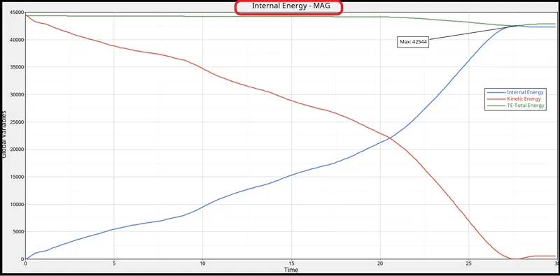
• This case is simmilar to case-1 difference is that here is only one notch in middle and in case-1 two types of notches was there on tube so the graph variation will be approx to case-1.
• Since due to one notch edge to edge interaction will less than first case thats why deformation is little less so incraese in internal energy is also less than first case.

Rigid wall force-

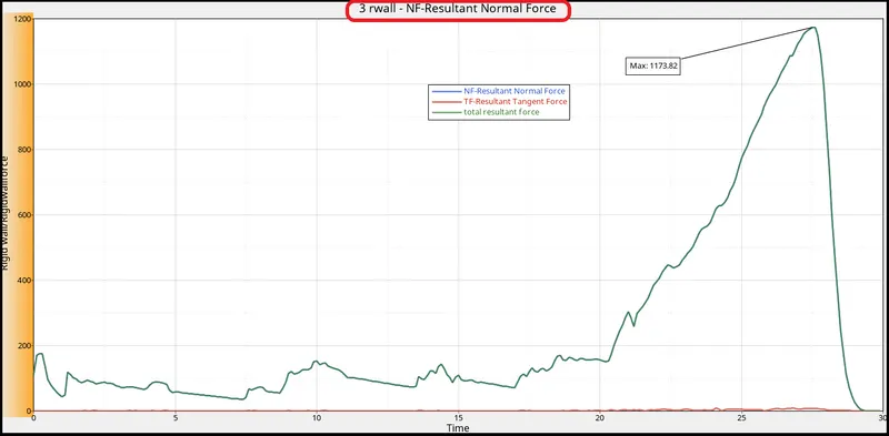
• Rigid wall force is also follow the same pattern as case-1 and maximum value will be less than first case is because of notch at only one place in this case.
• There will be drop in maximum value compare to previous case(case-4).
• This drop is observed due to removal of boundary condition.

Contact energy-

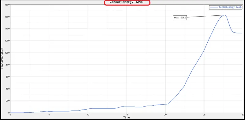
• Due to notch increase in contact energy we can see.Due to notch friction between elements will be more hence contact energy increased compared to previous case(case-4).

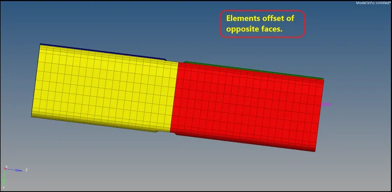
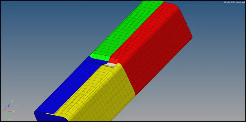
Case-6 :Create a new notch with nodes only from opposing 2 faces and run.

• Create notch using element offset methode.Go to 2D > Element offset.

•  Now run the simulation and save the radioss file as different case as case-6.
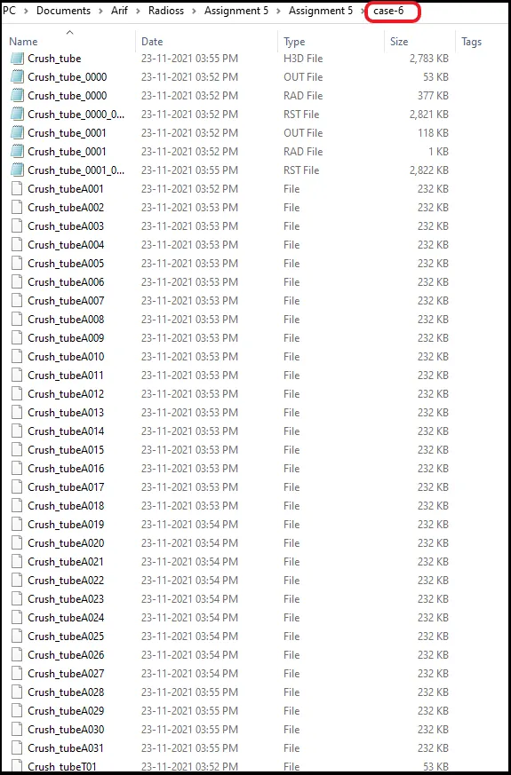
• After running the simulation we will get animation file, h3d file and also T01 file.

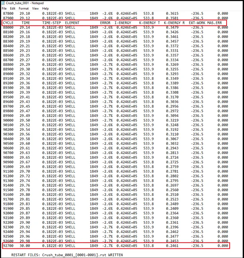
• Now open 0001.out file and check all the details. 
• Here we can see all variable in the out file about energy and mass loss also.
• So for checking the maximum loss check the last cycle details.

Post processing-

• Review the simulation using Hyperview.
• Plot the graphs using Hypergraph-2D

1.Review the simulation using Hyperview.

• Now after importing the h3d file on hyperview GUI go for contour activation.
• In contour it will show the simulation graphically and contour lies of load and other properties variation.
• To activate contour go to Tool bar > contour as shown below.
• Go to Contour > von-mises > averaging methode as simple > apply contour.

 

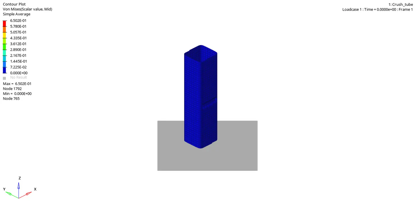
• simillarly for plastic strain-

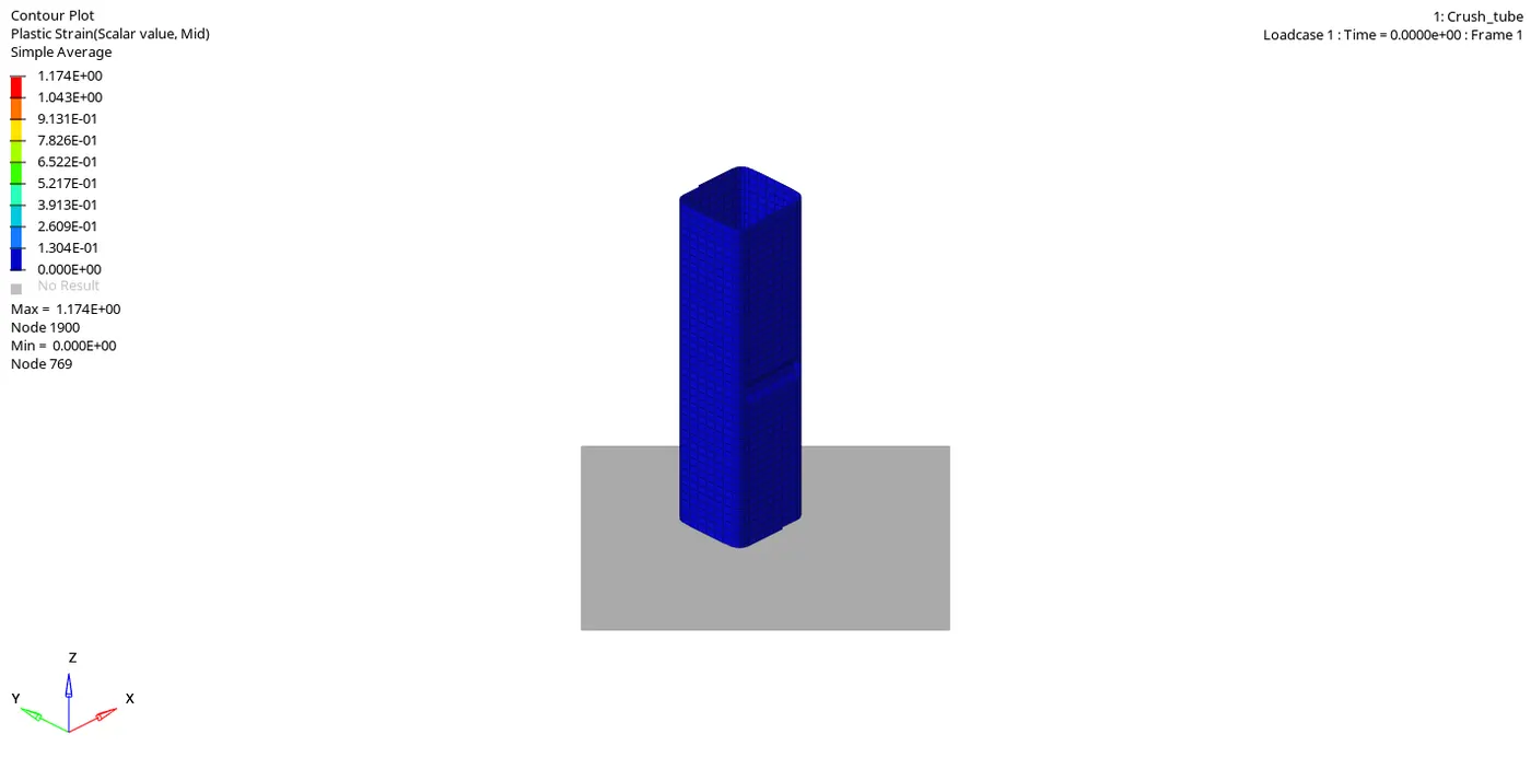
• In this case also deformation will start from notch area.And von-mises and plastic stain value will decrease compared to previous case.
• Because in this case notch area is less compared to previous so that stress value is less.

2. Plot the graphs using Hypergraph-2D

• Now split the window in 3Part and open hypergraph-2D in new window.
• After opening the hypergraph window import the T01 file in Hypergraph.

Go to Global Energy > Kinetic energy+Internal Energy+Total energy > Magnitude > solver unit > apply.

Global Energy graphs-

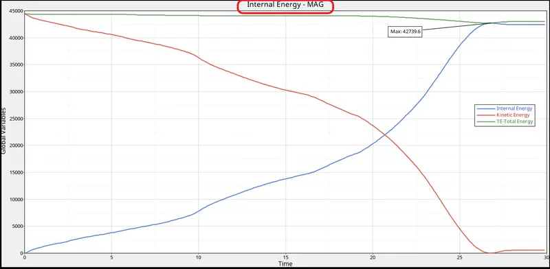
• Gain in internal energy is more than previous case because here continous deformation due to less notch area. 
• So that max internal energy gain is more than previous case.

Rigid wall force-

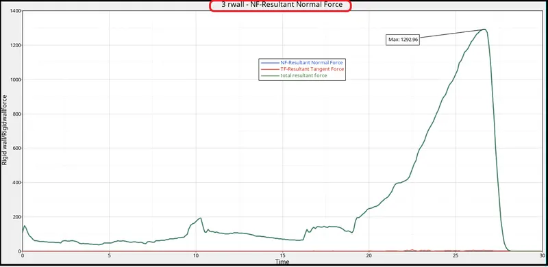
• Here rigid wall force will increase because of more deformation, so that more no. of element are are applying force to wall. 

Contact energy-

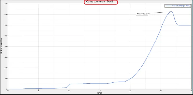
• Here contact energy will decrease than previous case because the amount of friction between meeting elements is less due to less notch are.

Cases	Energy  error	Internal Energy	Kinetic Energy	External work	Mass Error	Elapsed time	Total no. of cycle	Type of Interface used.	Change in model.
Case-1	-3.8%	0.4202E+05	592.6	-105.2	0.000	108.56 s	83400	Type 7	No change,Deafault deck setup.
Case-2	-3.8%	0.4202E+05	592.6	-105.2	0.000	108.56 s	83400	Type 7	Activate Inactive-6 to avoid intital penetration.But there is no intial penetration already.
Case-3	-12.3%	0.3823E+05	558.1	-188.6	0.000	108.32 s	102000	Type 7 & Type11	Recomended parameters given to interface contacts.
Case-4	-3.1%	0.4228E+05	570.8	-169.3	0.000	109.95 s	80900	Type 7 & Type11	Notches removed to avoid stress concentration.
Case-5	-3.5%	0.4188E+05	609.4	-346.5	0.000	101.12 s	85300	Type 7 & Type11	Created one notch at middle to check the stress concentration behaviour.
Case-6	-2.7%	0.4246E+05	533.8	-236.5	0.000	110.68 s	92700	Type 7 & Type11	Notches created on opposite faces only not on fillet region.

Result-

• Bumper model is meshed successfully with 6mm size.
• Crash model is run with different parameters.
• All 6 cases is reviewed in hyperview.
• Graphs for all cases in drawn in hypergraph 2D.
• Maximum and minimum value variation of is analysed with all case.
• Hence results of all cases compared successfully.

Learning outcome-

• In this challenge i came to know the different kind of contacts intefaces.
• Also learn to apply parameters for contacts and their effects on simulation results.
• I came to know that the stress conecntarion behaviour with notch present in any model.
• The element deformation and self contact behaviour of FE.