Contact Interface Modelling using Type7 and Type11 in Hypermesh
Assignment 5 Report.
- Objective: To successfully complete and understand the following two studies given:
Study1: Creating a 2D Mesh on the given Bumper Assembly System.
Study2: To change the Contact interface properties of the given model and compare the results by plotting various graphs of the outcome. - Procedure:
Study1: To create a 2D Mesh on the bumper Assembly.
1. In the very first study that we have, we need to Mesh the component. To begin with the Meshing of the component, we initially need to clean the geometry of the given mid surface. We can see the errors in the File such as the following: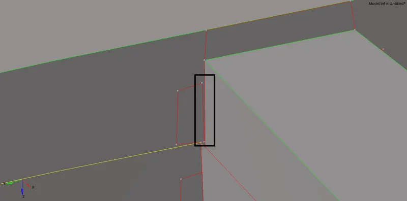
Surface Error.
Now to fix this error we need to use the Toggle command. To use this command, we need to use the Quick Access command (shortcut-F11). In this tab, we need to use the Toggle edges option as shown. This command will basically join the lines together.
Toggle Edges command.
Before toggling the edges, we also need to increase the tolerance of the toggle command.
The final output will look something like the following: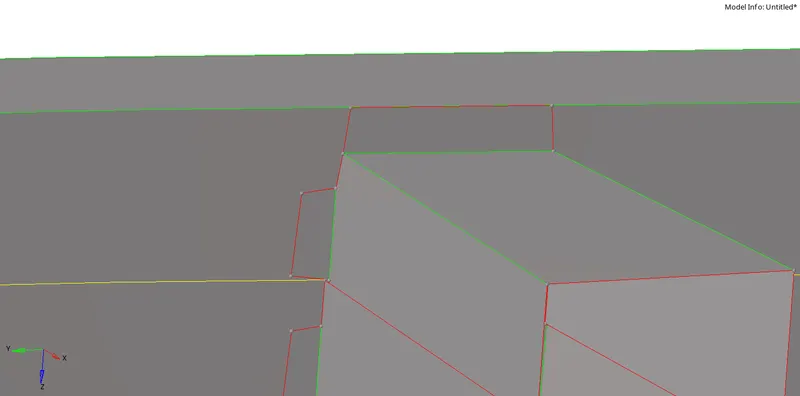
Cleaned up surface.
Like this, we need to clean up the Geometry of the entire component. This procedure is known as the Geometry Clean Up of the model. After this process, we then proceed to mesh the component.
2. To mesh the component, we need to use the Automesh Command in the 2D Tab.
2D -> automesh.
We need to give the Average element length as 6.0mm as mentioned. It is also a good practice to check the Flow Align option as it will give a much better mesh flow and mesh alignment.
Automesh Command.
We then mesh the entire component from surface to surface and get a final output, something like the following: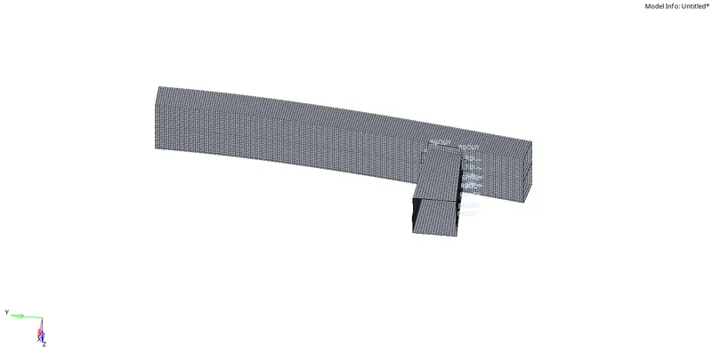
Final Meshed Component.
3. The final Step in meshing this model is to add a Rigid Body Connection wherever the surfaces are not properly connected. To add an RBE2 connection to it, we need to use the Rigids command under the 1D tab. This command will create an RBE2 connection that will distribute the loads equally amongst the nodes that are attached to it.
1D -> Rigids.
Rigids command.
The RBE2 connection will look something like the following: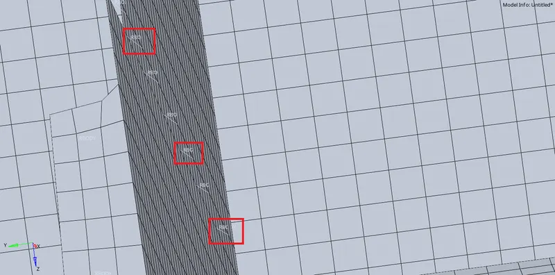
Rigid Connections defined
After the connections were made, we can then conclude that the Bumper System Model is Meshed properly.
Study2: To change the Contact interface properties of the given model and compare the results by plotting various graphs of the outcome.
There arevarious cases under this study. We will examine them one by one and then draw conclusions with the Graph plots of various energies and Forces from the simulation.
Case1: Default simulation (Type7 Contact Interface)
1. The first step is to import this model. To import this model, we need to use the import command and then use the file option in it. In this file option, we need to import the Starter File(The files with names ending in _0000.rad). Since the engine file is linked to the start file, any changes made will be saved.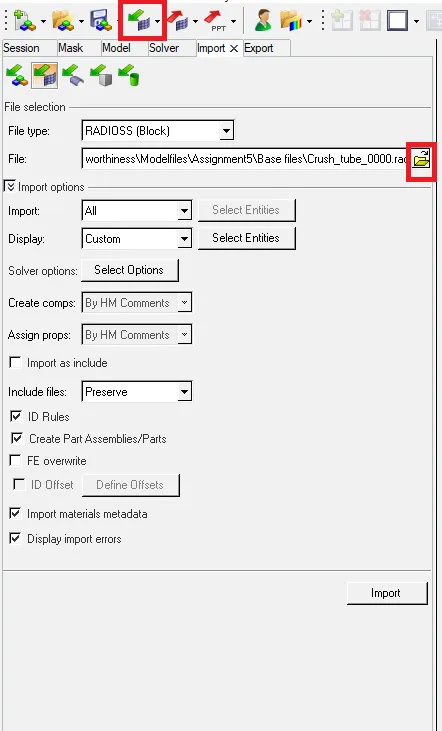
Importing a File.
2. In Case1, we have to run the base file as it is given. We can clearly see that the Contact interface is defined as Type7. To check the Contact interface defined, we need to use the Model tab and then use the Group card in it.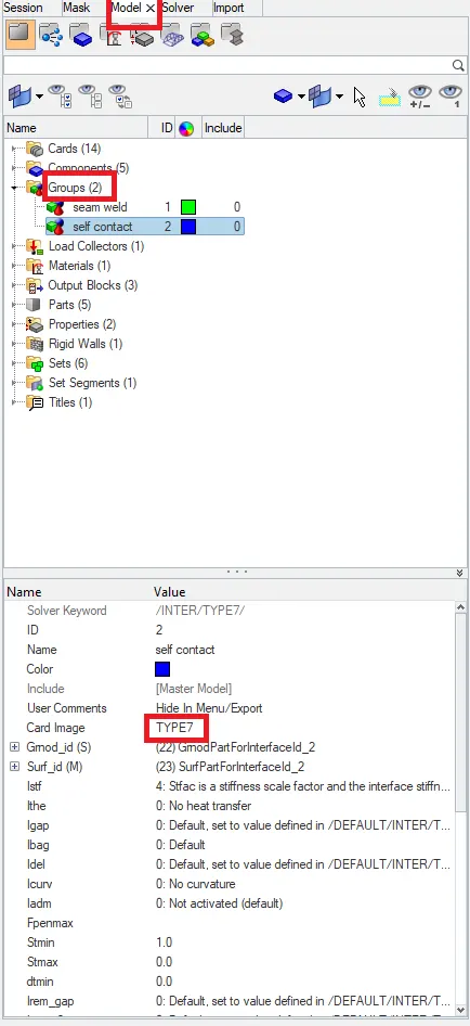
Type7 contact defined.
Now to run this simulation, we can use RADIOSS command in the Analysis tab. In this, we can save where the files are needed to be saved. We then click on the "RADIOSS" command and run this simulation.
Analysis -> RADIOSS
The input file location is the file location where all the animatin files and the Time History Files will be saved.
RADIOSS command.
3. After this, we then go on to see the Animation of the simulation results. To view the Animation, we need to change from Hypermesh to Hyperview as shown.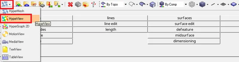
Hyperview Tab.
We then simply need to import the .h3d file in this tab as shown. This .h3d file is basically a combination of all the Simulation files that were created by the solver.
Importing the .h3d file
The simulation for Case1 will look something like the following: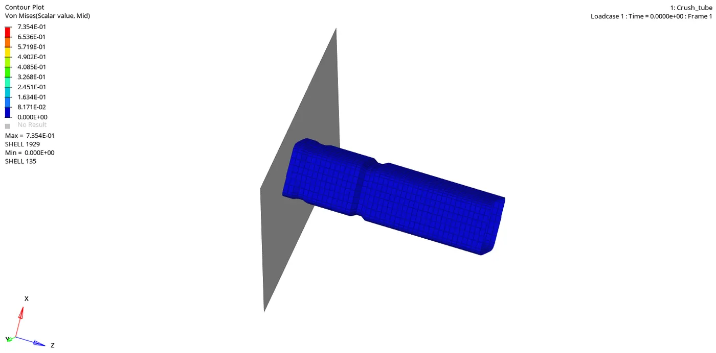
Von Misses Plot for Case1
The given plot is drawn for the Von misses stresses in the specimen. Similarly, we can plot Displacement and Contact energy plots on the Specimen. To do this, we simply need to change the contour plotting from Von missess to Displacement as shown:
In this method, we can plot the Displacement and the Contact Forces in the Specimen. The plots will look something like the following: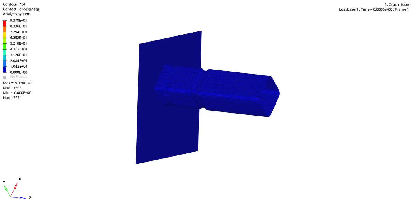
Contact Forces Plot for Case1
From the Contact forces plot, we can clearly see that the Forces are maximum when the entire specimen has failed(colour change).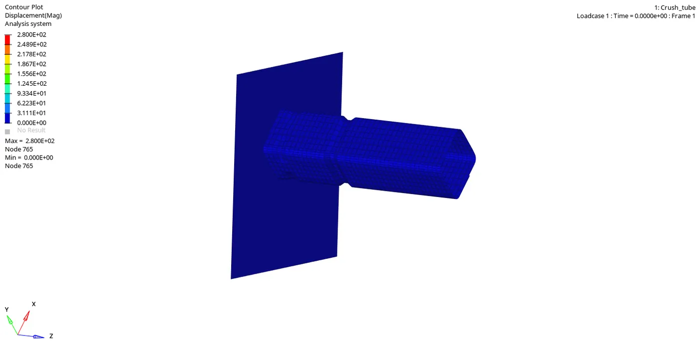
Displacement Plot for Case1
The Displacement Plot shows the Displacement of the Elements in the simulation. And the elements at the very end are having a much greater displacement than the elements that are near the wall. This displacement can be considered as the deformation of the elements as well. So, the elements that are at the end are deforming much more than the elements near the wall as the simulation is progressing.
4. The next step is to plot the required graphs for this case. We need to use Hypergraph. We can switch to Hypergraph from the same tab as how we switched to Hyperview. In the Hypergraph tab, we need to input the Time history File for the simulation. This time histroy file has all the data points that we have requested the solver to extract from the simulation. From this file, we can plot any graph required.
We can import this file using the shown option.
Importing the Time History File
After this, we can select the quantity that we want to be plotted. Like this we can plot the following Graphs: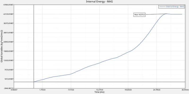
Internal Energy Plot.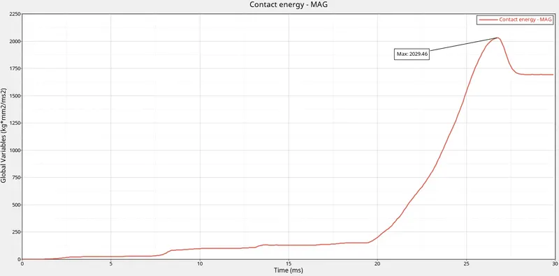
Contact forces plot.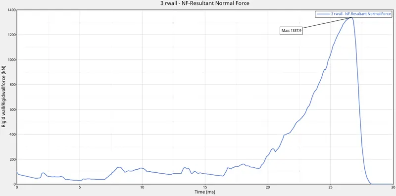
Rigid Wall Forces Plot.
All these graphs represent information regarding the simulation.
In the Internal Energy plot, we can see that the curve is continuously increasing and then flatens out after around 26.5ms. We can understand that as the Deformation in the Specimen is continually increasing, the internal Energy is also increasing. But after a specific point in time(around 26.5ms) the Deformation in the specimen cannot increase anymore as the specimen has failed after this point.The maximum magnitude that the Internal Energy touches is around 42270mJ After this point, there is no more deformation possible in the specimen and hence the curve also flatens.
In the Contact Energy plot, we can understand that as the simulation progresses, the contact between the specimen and the Rigid wall increases and hence the contact force between them is also Increasing as indicated by the graph as well. But after a particular point in time, the Contact is being lost(can be seen in the simulation) and hence even the curve drops in magnitude and flatens after that point. The extreme value for Contact Energy is 2030mJ and then it reduces to approximately 1700mJ and then the curve flatens.
In the Rigid Wall Forces plot, the forces are being plotted are the Normal Forces that the Rigid Wall is applying on the Specimen. So, as the contact energy is increasing, the Rigid Wall forces will also increase, and at the point where the Contact energy flatens out, we can see that the Rigid Wall Forces also decrease and eventually when the specimen loses contact with the Rigid Wall, the Rigid Wall Forces become Zero. The peak magnitude of the Rigid Wall forces is around 1350kN.
Case2: Change the Inacti = 6.
Inacti Formulation defines the action that the solver needs to take if there are any pre-existing penetrations present in the model. Inacti=6 is the recommended formulation as it reduces the gaplength by an extra of around 5% of the difference between the original gap and the penetration length. So to change the Inacti length, we must use the Groups Card and then use the Properties of the Self contact and then change the Inacti value there.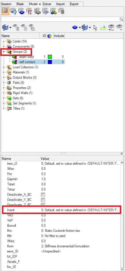
Inacti = 6
Here, we need to change the value of the Inacti formulation to 6 and then run the simulation.
We will get the Simulations something like the following: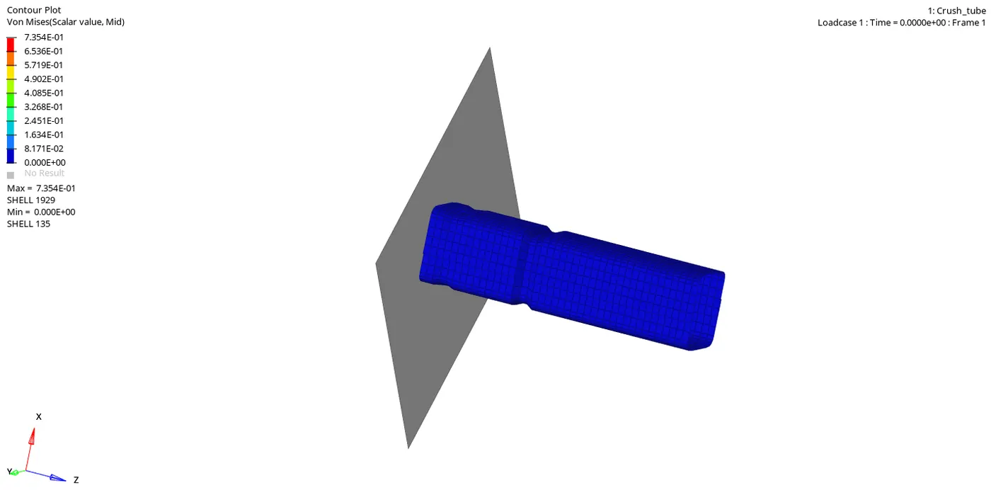
Von Misses Plot.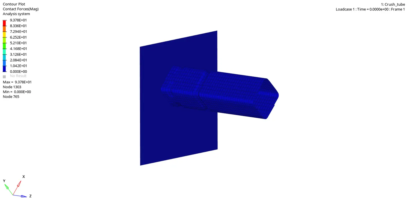
Contact energy plot.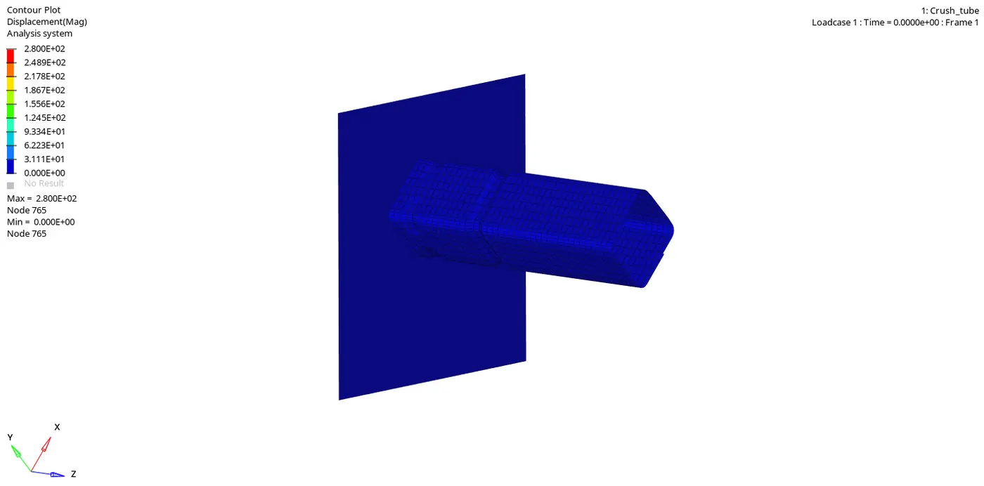
Displacement Plot.
In this simulation, the Displacement Plot indicates the displacement of the components. And the elements have a much higher displacement at the very end than the elements that are near the wall. It is also possible to consider this displacement as the deformation of the elements. So as the simulation progresses, the elements which are at the end deform much more than the elements near the wall.
The Graph of the Simulation will be like the following: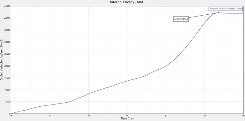
Internal Energy
Contact Energy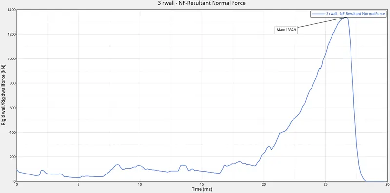
Rigid Wall Forces.
We can understand in the Contact Energy plot that the contact between the specimen and the Rigid wall increases as the simulation progresses, and thus the contact force between them also increases as shown by the graph.But the contact is lost (can be seen inthe simulation) after a certain point in time, and thus even the curve drops in magnitude and flatens after that point.
The forces being plotted in the Rigid Wall Forces plot are the Usual Forces applied to the Specimen by the Rigid Wall. So as the contact energy increases, the Rigid Wall forces will also increase, and we can see that the Rigid Wall Forces also decrease at the pointwhere the Contact energy flatens out and finally when the speciment loses contact with the Rigid Wall, the Rigid Wall Forces become Zero.
- The maximum magnitude that the Internal Energy reaches in the simulation is around 42300mJ and then once the maximum deformation in the model is reached, then the curve flatens out.
- In the Contact energy plot, the maximum value during the entire simulation is 2000mJ and once the maximum strain rate is achieved, the value drops down to approximately 1700mJ.
- In the Case of Rigid Wall forces, the maximum magnitude is reached at around 1350kN and then as the tube loses contact with the rigid wall the value decreases to then eventually zero.
Case3: Creating a Type11 contact and running the simulation.
So, to create a Type11 Contact, we can change the Type7 contact interface into type11 contact. After changing the contact type, we then need to feed in the Recommended properties into the software.
The recommended properties are as follwoing:
1. Igap = 3 (Variable Gap taken into account.)
2. Gapmin `>=`0.5mm (minimum thickness to avoid numerical issue.)
3.Inacti = 6 (remove initial penetrations wherever possible, else reduce to less than 30% of the defined gap)
4. Istf = 4 (Stifness based on softer Segment)
5. Stmin = 1000 N/mm (Minimum stiffness in contact to avoid too soft contact.)
6.Idel = 2 (remove slave nodes from contact because of element deletion)
7. Iform = 2 (Frictional Forces are calculated on the basis of Stiffness parameter.)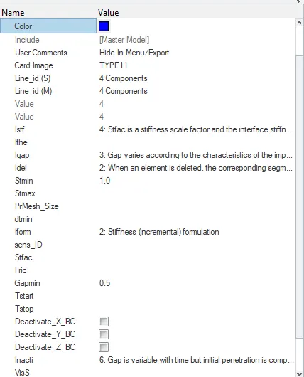
Type11 Contact created.
We can input these properties using the Groups card in the Model tab as shown earlier. after these properties were given as an input, then we need to run this simulation.
We get the simulation result as the following: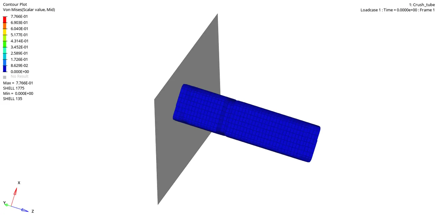
Von Misses Stress Plot for Case3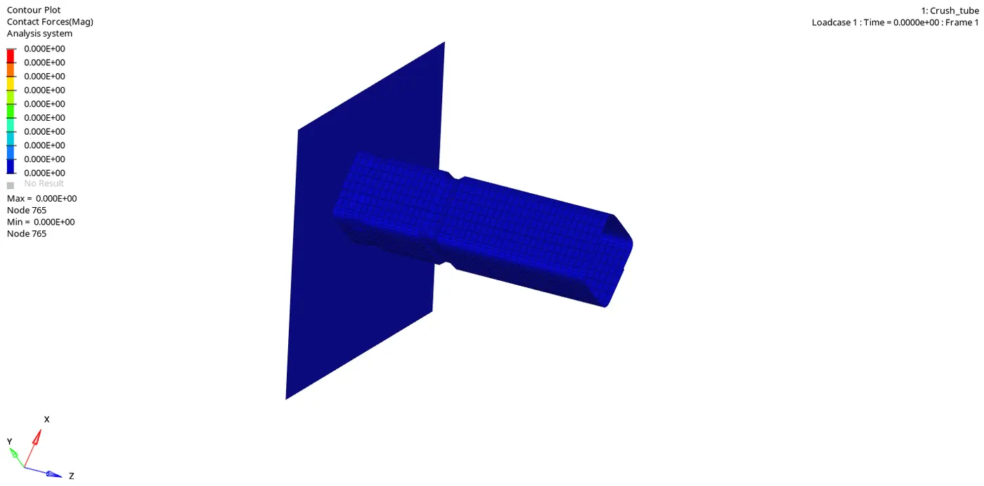
Contact Forces Plot for Case3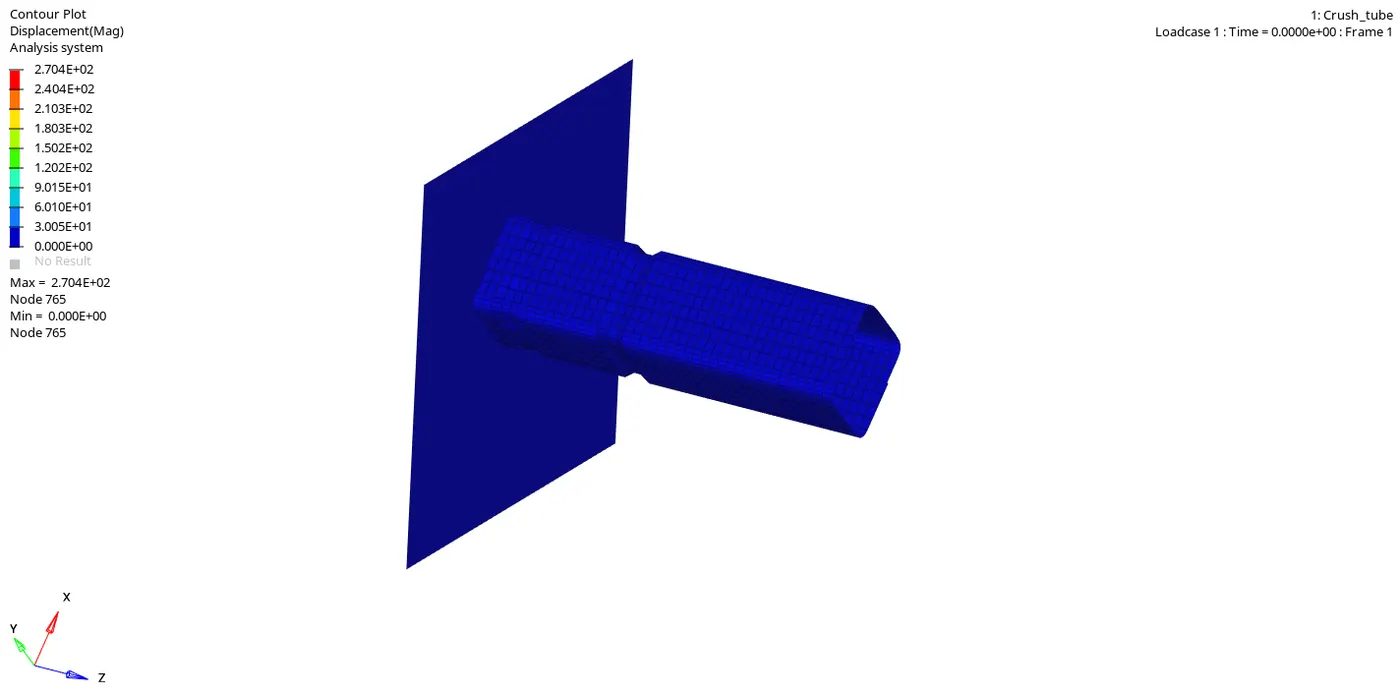
Displacement Plot for Case3
We can plot the graphs for the same. The plots for this case are as follows: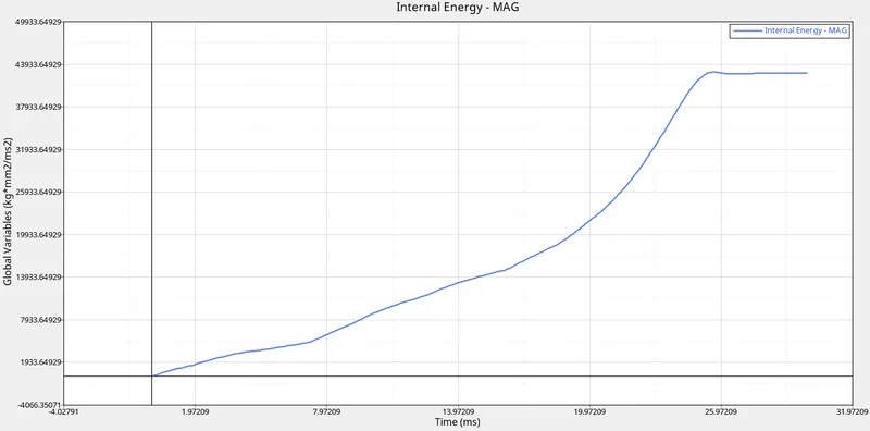
Internal Energy Plot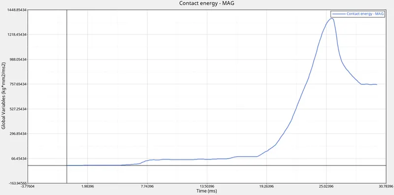
Contact Forces Plot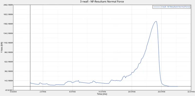
Rigid Wall Forces.
From the Internal Energy plot, we can understand that as the simulation progresses, the deformation in the elements is increasing and hence the internal energy is increasing. After a particular point in time, there cannot be anymore deformation in the Tube and hence the curve also flatens and tries to become constant.
Even with the contact energy plot, we can see that as the deformation is increasing with the progressing simulation, there is an increase in contact between the Rigid Wall and the Tube. As the contact increases, we can see an increase in the Contact energy and the Rigid Wall Forces. And when the tube loses contact with the Rigid wall, the curve also slopes down and the magnitude also decreases. But in this case,
- The peak value of the Internal energy in the simulation is around 43000mJ and once the maximum strain rate is achieved, the curve flatens out.
- The maximum magnitude of the Contact Energy is around 1370mJ and once the peak deformation is reached the value drops down to 754mJ before the curve completely flatens out.
- In the case of Rigid wall forces, the peak magnitude achieved is 1650kN.
Case4: To Remove both the notches and the given Boundary condition on the Master node of the Rigid Body connection.
A notch can be defined as an indentation on the surface that will give like a depth to a portion on the surface. Its like a groove or a cut on the surface.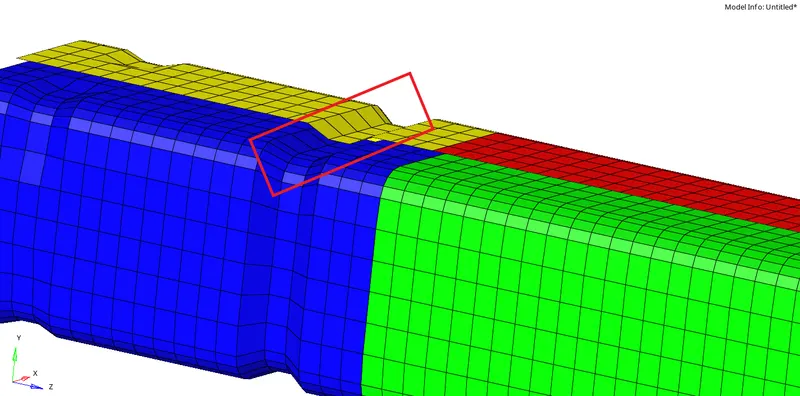
Example of a notch.
So, in our tube specimen, there are two notches present on the surface. So in the fourth case, we need to remove the notches. To do this, we simply need to use the Translate command (shortcut- shift+F4) in the Tool tab.
Tool -> Translate
Translate command.
In this command, we basically uplift the nodes that are at the bottom of notch to the plane of its respective surface. We select the nodes and then give the magnitude by which we want the nodes to be uplifted. Then we need to select the N1,N2,N3 which are just nodes that will help us define a plane along which we want the nodes to be lifted up.
Using this procedure, we can remove the notch along all the faces in the tube, and the specimen will look something like the following: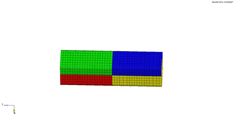
Notch was removed.
After the notch was removed, the next step was to remove the boundary conditions on the Rigid Body connection. To do so, we simply need to use the Solver tab and then use the "BCS" card and uncheck all the Degrees of Freedom that were pre-set.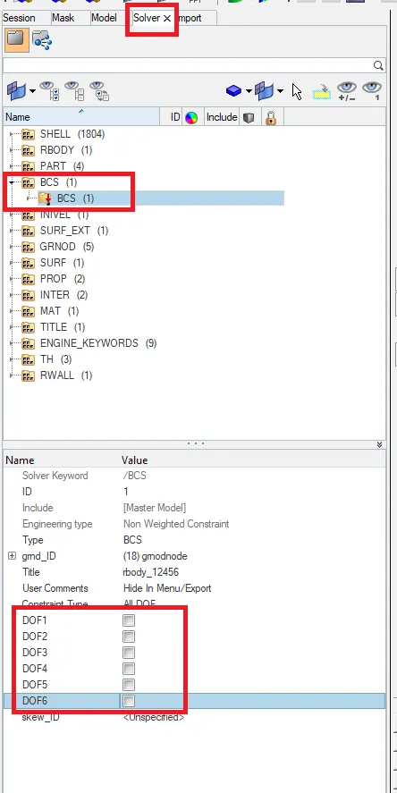
Boundary Conditions removed.
After all the setup for the case was done, we then go onto run the simulation. the simulation will look something like the following: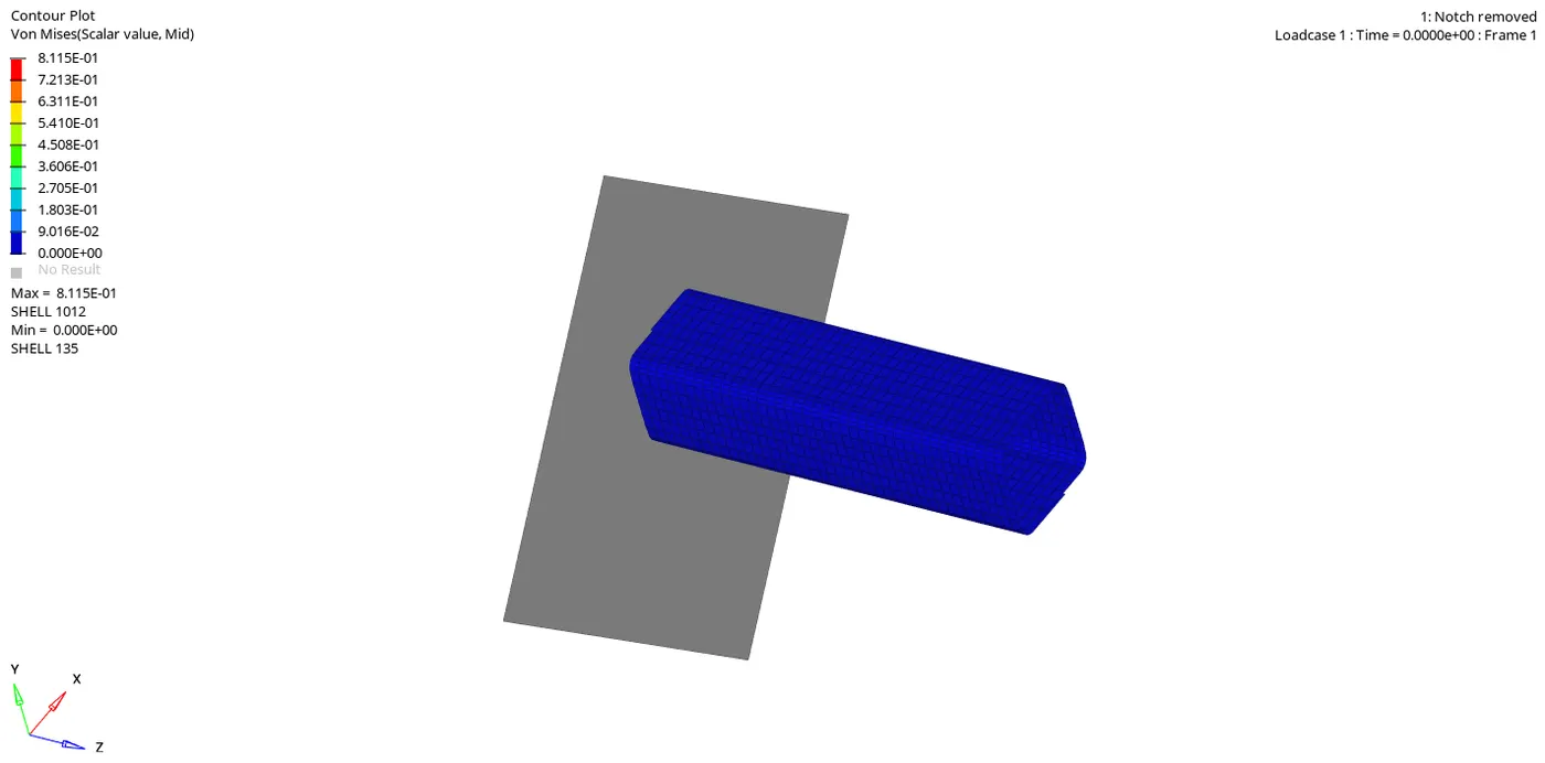
Von Misses Stress Plot for Case4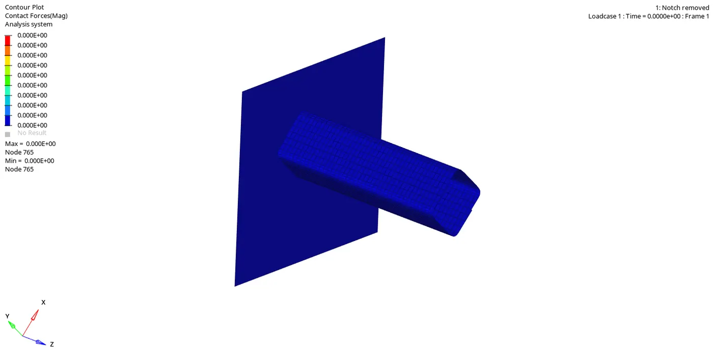
Contact Forces Plot for Case4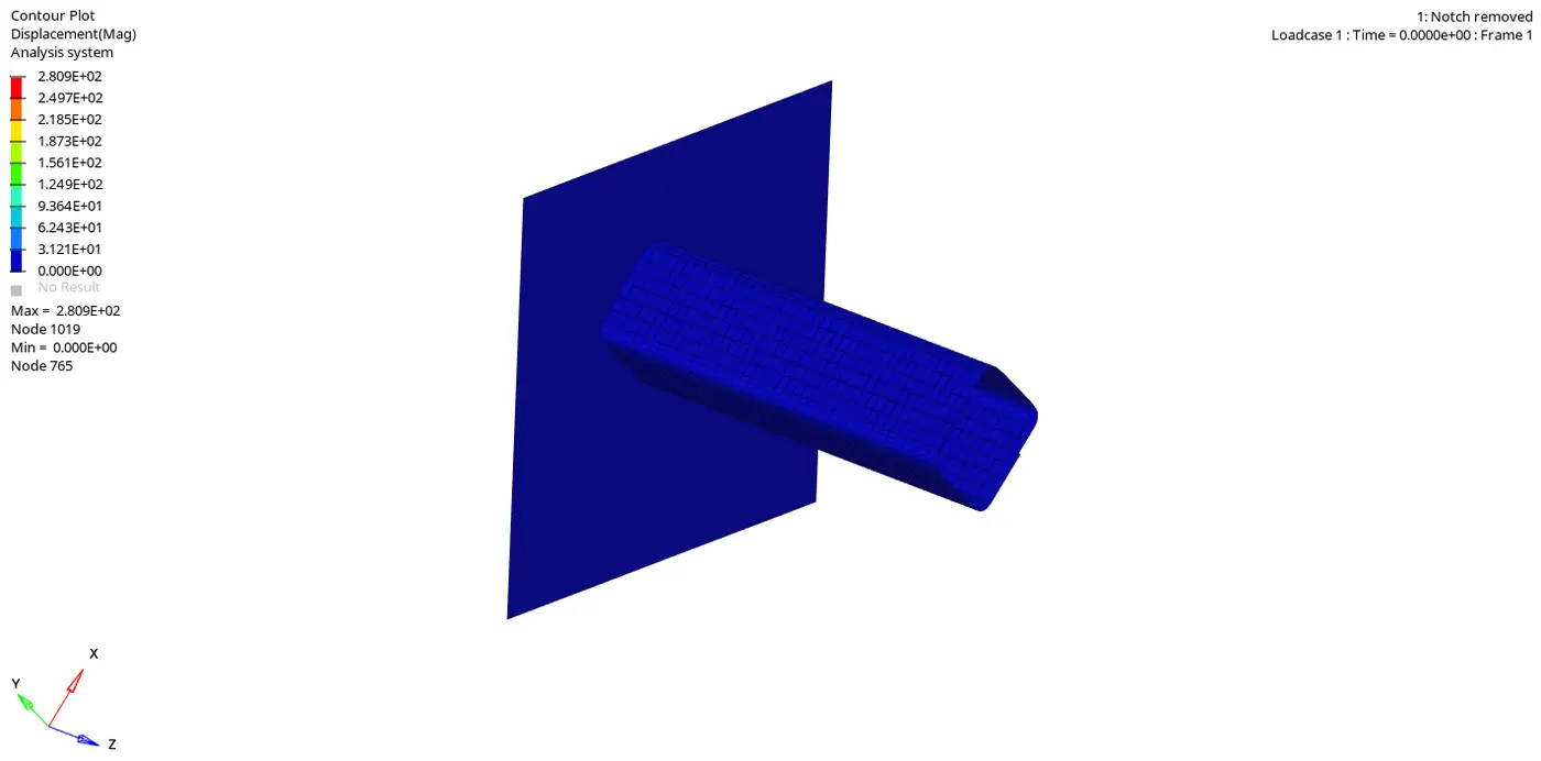
Displacement Plot for Case4
These are the simulation, we can even see the maximum and minimum values in it.
We then go on to plot the various graphs for this simulation: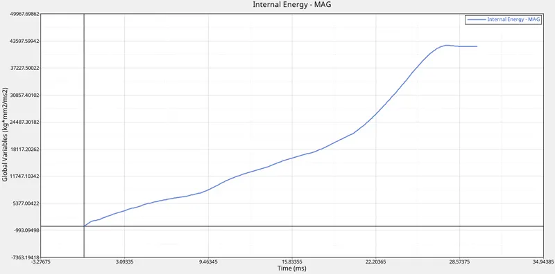
Internal Energy Plot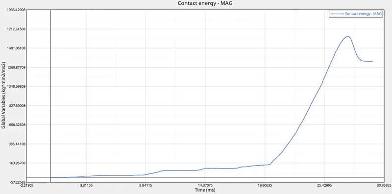
Contact Energy Plot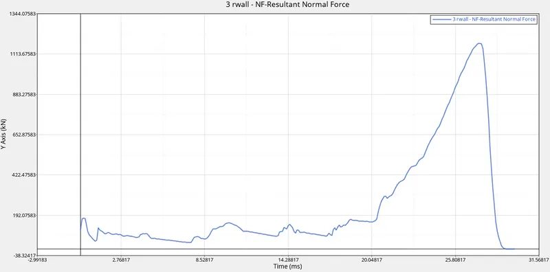
Rigid Wall Forces.
- The peak value of the Internal energy in the simulation is around 42500mJ and once the maximum strain rate is achieved, the curve flatens out.
- The maximum magnitude of the Contact Energy is around 1630mJ and once the maximum deformation is reached the value drops down to 1350mJ before the curve completely flatens out.
- In the case of Rigid wall forces, the peak magnitude achieved is 1200kN.
Case5: Creating a Notch in the middle of the specimen
To create a Notch in the middle of the Specimen, we need to basically translate the nodes in the downward direction. We need to select the nodes and then select the plane along which we need the nodes to translate. We then give in the Magnitude and translate the nodes. The final output of the created notch will look something like the following: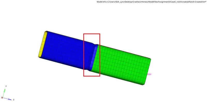
Notch Created.
After the Notch was created, we then go on to simulate the model. The simulation results are shown below: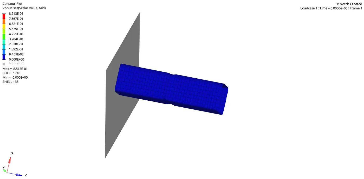
Von Misses Stress Plot for Case5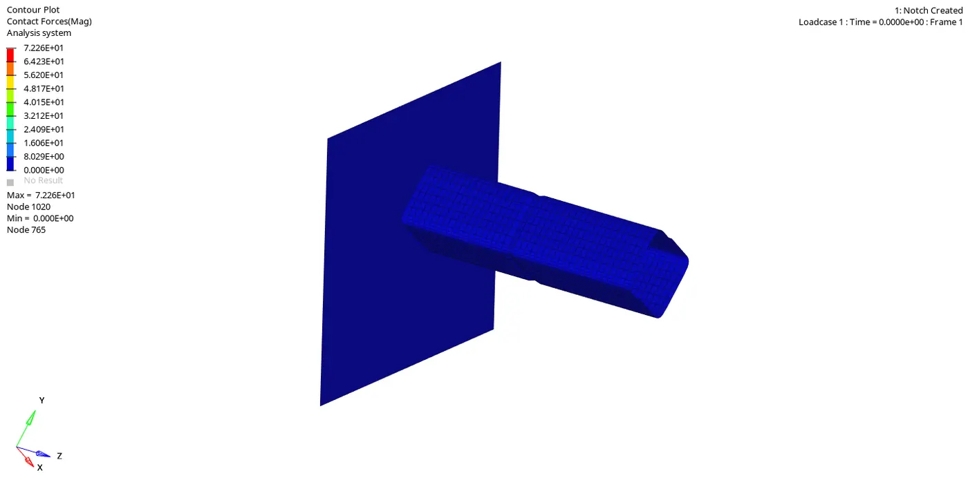
Contact Forces Plot for Case5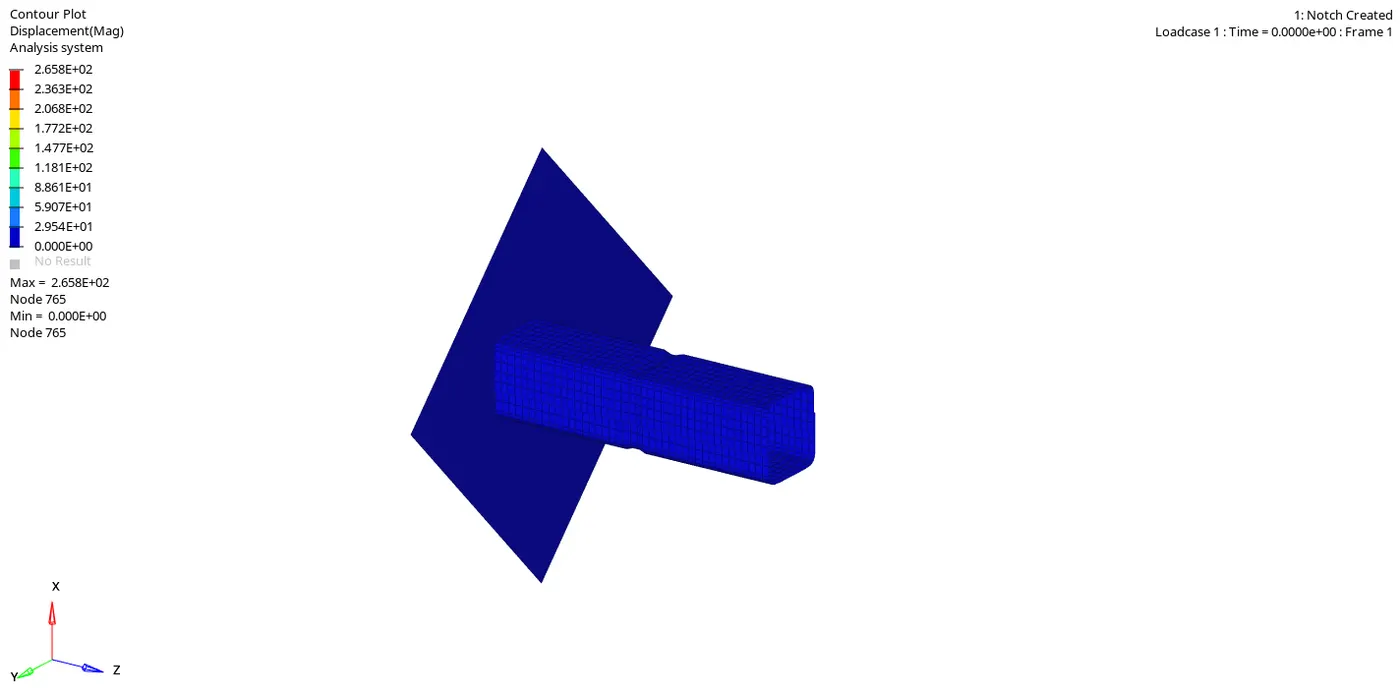
Displacement Plot for Case5
In this simulation, the Displacement Plot indicates the displacement of the components. And the elements have a much higher displacement at the very end than the elements that are near the wall. It is also possible to consider this displacement as the deformation of the elements. So as the simulation progresses, the elements which are at the end deform much more than the elements near the wall.
The graph plots of different Quantities are as follows: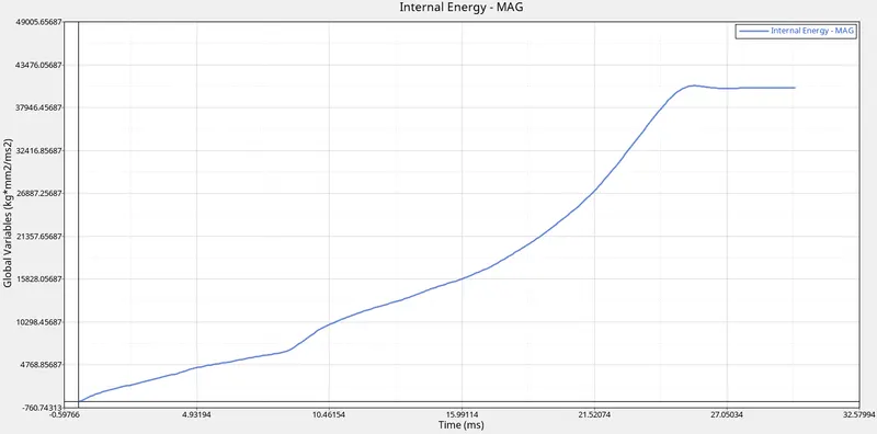
Internal Energy Plot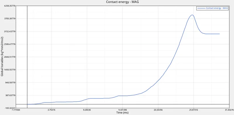
Contact Energy Plot.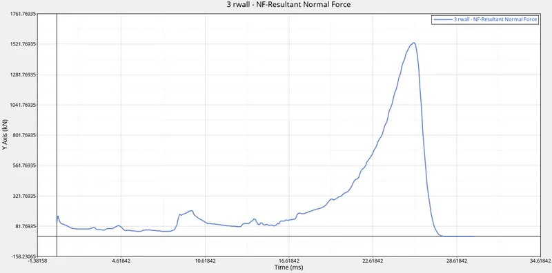
Rigid Wall Forces.
- The peak value of the Internal energy in the simulation is around 41000mJ and once the maximum strain rate is achieved, the curve flatens out.
- The maximum magnitude of the Contact Energy is around 3850mJ and once the maximum deformation is reached the value drops down to 3000mJ before the curve completely flatens out.
- In the case of Rigid wall forces, the peak magnitude achieved is 1530kN.
Case6: To create a notch on any two opposing faces
So in this case, we only notches on any two opposing faces. So to fulfil this condition, we can simply remove the notches from any two opposing faces and then proceed to simulate the model. We can remove the notches in the exact same manner as how we did in Case4.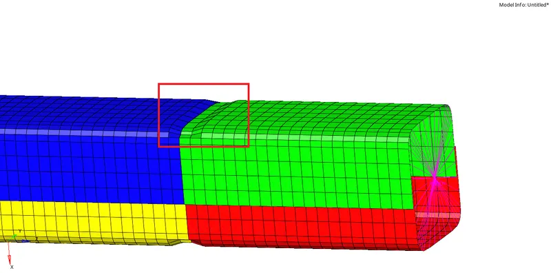
Notch Created
After the notches were removed, we then go on to simulate the model. The different simulation plots will look something like the following: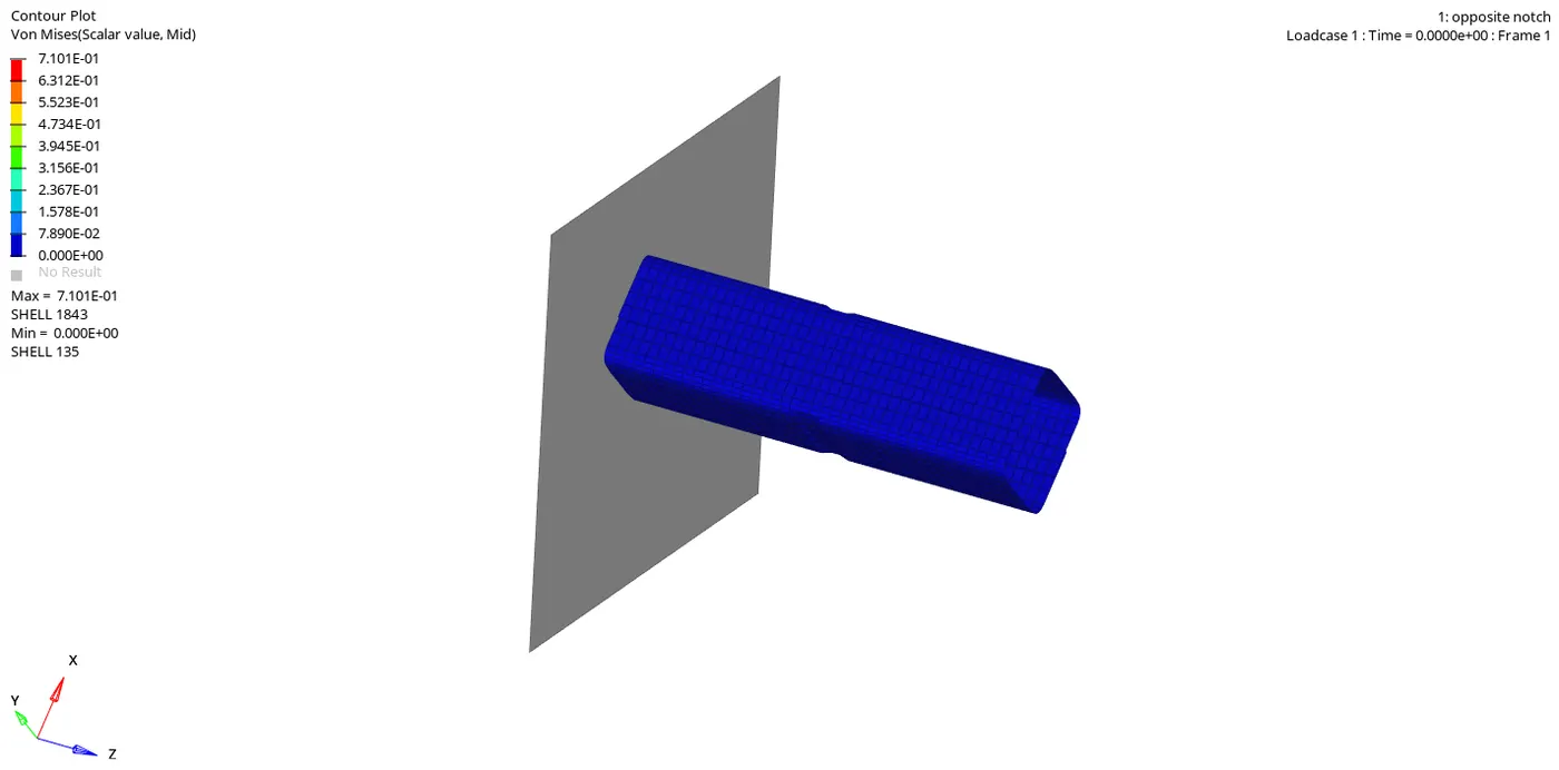
Von Misses Stress Plot for Case6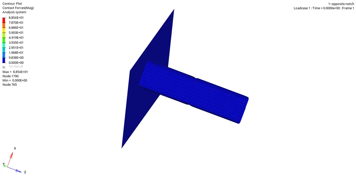
Contact Forces Plot for Case6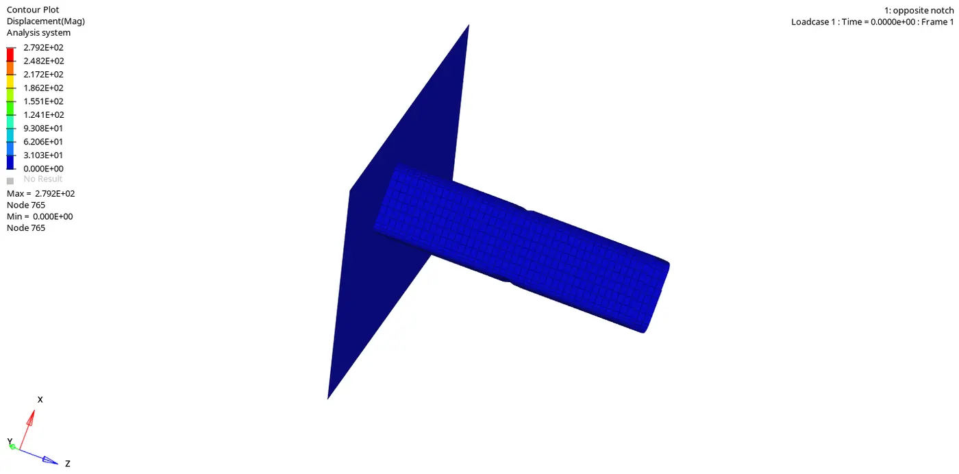
Displacement Plot for Case6
The next step would be to plot the graphs of all the different quantities in the simulation. The plots will look something like the following: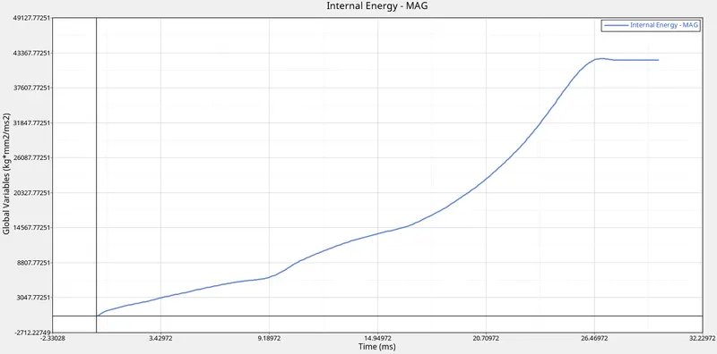
Internal Energy Plot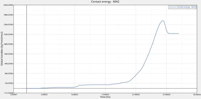
Contact Energy Plot
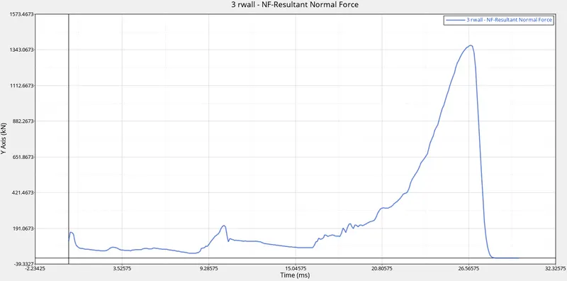
Rigid Wall Forces.
- The peak value of the Internal energy in the simulation is around 42550mJ and once the maximum strain rate is achieved, the curve flatens out.
- The maximum magnitude of the Contact Energy is around 1700mJ and once the maximum deformation is reached the value drops down to 1350mJ before the curve completely flatens out.
- In the case of Rigid wall forces, the peak magnitude achieved is 1380kN. - Comparison between different cases:
Case1 and Case2: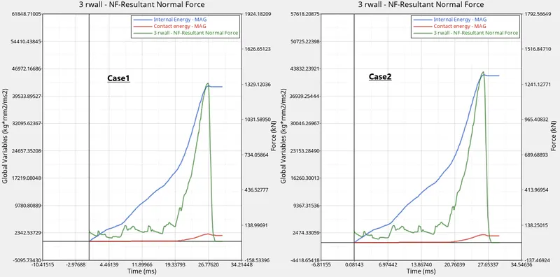
Graph for Case1 v Case2
We can see and compare the difference in the amount of energies that were recorded during the simulation. In Case1 we can see that the Internal Energy is around 42500mJ whereas in Case2 it was recorded as 42300mJ. In the magnitude of The Contact energy and the Rigid wall forces, there is not much of a difference between them. In both Case1 and Case2, we have recorded a Contact Energy of 2000mJ and a Rigid Wall Force of 1350kN.
In terms of the property changed, we have only changed the property of Inacti and changed the value of it to 6. Since there were no penetrations in either Case1 and Case2, we do not observe a significant change in the energy values.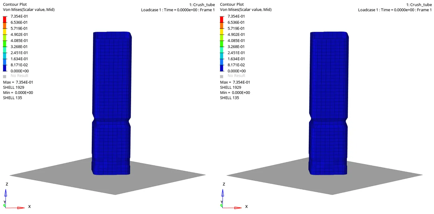
Simulation for Case1 v Case2
Case3 and Case4: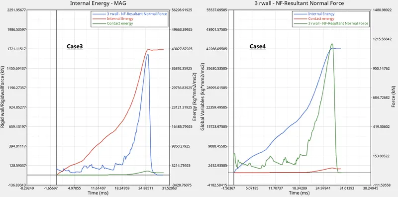
Graph for Case3 v Case4
We can see a change in the energies when we compare these two cases. In the case of Internal Energy in the two cases, the peak values are very much comparable. In case3 the Internal Energy peaked at 43000mJ and in Case4 the energy peaked a 42500mJ. But when we compare the Contact Energies of the two cases, we can see a different scenario. In Case3, the Contact energy touched 1370mJ but on the contrary, in Case4 the Contact energy touched 1630mJ. This indicates that the elements in Case4 were deformed more and came into contact with each other more. This can be confirmed with the simulation attached below. In Case4, the deformation is also much more uniform as well. In Case3, the specimen starts to buckle earlier than in Case4.
Since we have removed the notches and the Boundary conditions, we get a lesser value of Rigid Wall forces.
From this we can conclude that Notches help in creating a region of Stress Concentration in the specimen and when we remove the notches, the specimen is bound to fail earlier.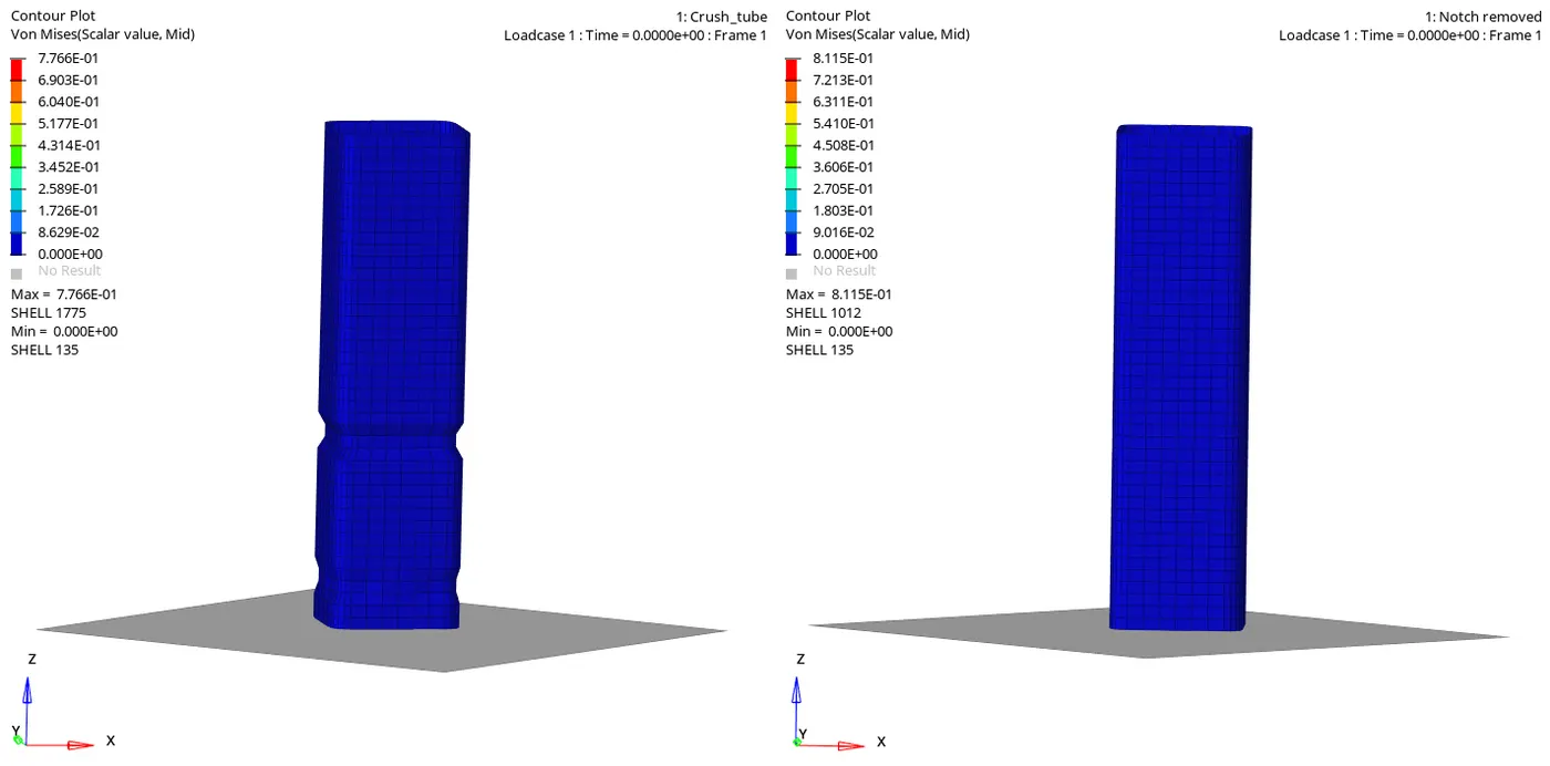
Simulation for Case3 v Case4
Case5 and Case6: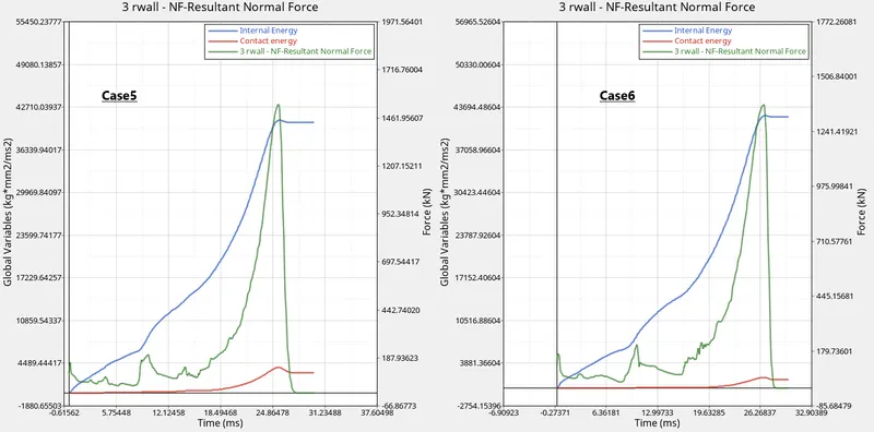
Graph for Case5 v Case6
We can see a difference in the internal energy of the two cases. In Case5 we have the Internal Energy peaked at 41000mJ but whereas in Case6, the internal Energy has peaked at around 42500mJ. And when we compare the Contact energies of the two cases we have a different view. In Case5 we have an Contact Energy of approximately 3880mJ but whereas in Case6, we have the contact energy peaked at 1700mJ. From this, we can infer that in Case5 we have much more deformation than in Case6. In the Rigid Wall Forces for both the cases we see it decreasing from 1530kN in Case5 to 1380kN in Case6. This can indicate that the Specimen is applying more force onto the Rigid wall in Case5 than in Case6.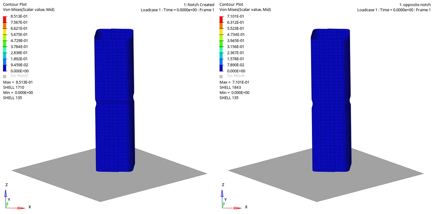
Simulation for Case5 v Case6 - Conclusion: In conclusion I would like to state that this assignment helped me understand the basics of all the energy mapping and how the contact interface will affect the Simulation of given component. In this assignment I revised how the meshing of a given component can be done as well.