Assignment 4-RADIOSS Material Laws Challenge

OBJECTIVE

To apply various cases in the given failure Johnson cook with law2 and law27 material and also doing simulation with plotting the graph and to compare the results.

PROCEDURE

CASE 1

In this case for the given .rad file, we’ll do a simulation without any changes in the material and property card. For the safer check the property card for element formulation. Here we don’t need to change anything.

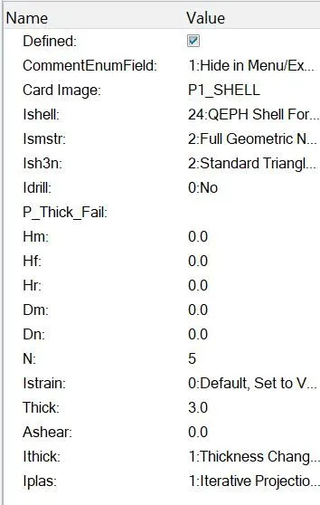
Import the model in radioss, after checking the property run solver with -nt 4 cpu commands. try saving the files in seperate folder and the solver will run the simulation on the solver console window. after the simulation open the hyperview window to view the animation of the simulation.

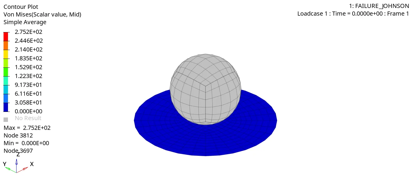
open hyperview window and import h3d file from the results. then switch to contour and gives vonmises to display. SInce the plate is law2 and this image shown that max von mises and elements which are deleting form the plate.

ENERGY ERROR

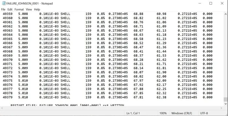
the energy error is 0.8%, internal energy is 0.2730E+05, mass error is 0, and number of cycles taken is 49379.

now we need to plot graph for all the resulted files. change it to hypergraph 2D and new window will appear. Import to1 file in the data file box. then plot rigid forces in the window.

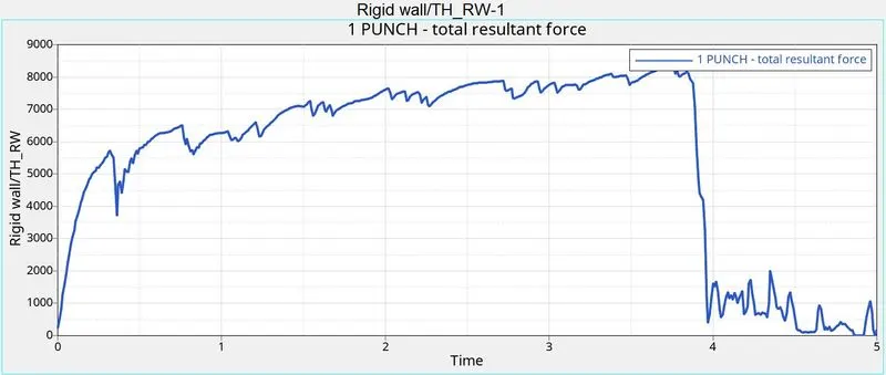
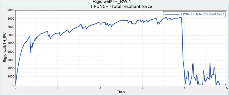
the increasing rigid forces is due to the starting time of the spherical ball hitting on the plate. at the final bending stress of the plate elements elements are deleting from the plate, so we can examine the graph drops after 4 second.

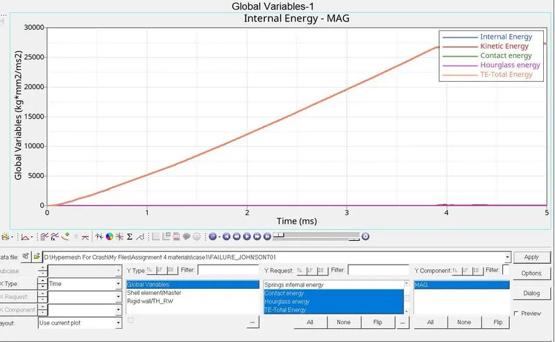
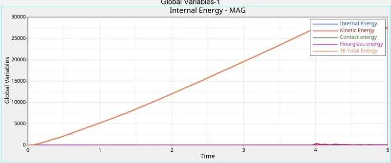
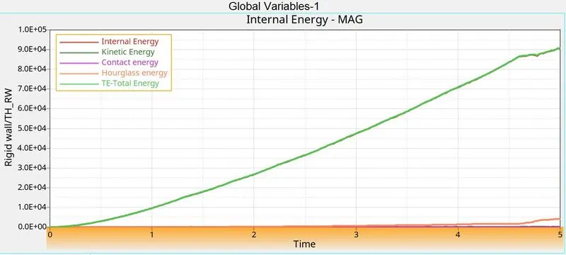
Now we will plot all the remining energies in the graph as internal energy, contact energy, hourglass, total energy. here we have no hourglass energy than internal and kinetic energy at increasing rate.

CASE 2

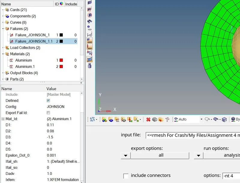
In this case failure card is edited with the given values. the material law for the material law2 is same. and the given values is Ifail_sh=1(default), Dadv=1, Ixfem=1 for the below images, and rename it as law2_epxmax_crack.

now the time to run the simulation with -nt 4 cpu's commands. this should be saved in a seperate folder for the final comparison.

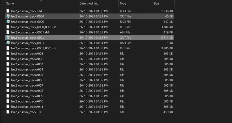
after the simulation open the 0001.out files to view the energy error of the simulation

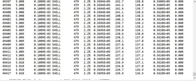
here energy error is 2.2%, internal energy=0.5694e=05, kinetic energy=236.6, mass error=0.000, total number of cycles=49417.

now switch it to hyperview to animate the simulation. import the h3d file and click apply. give shaded mesh elements to view the elements.

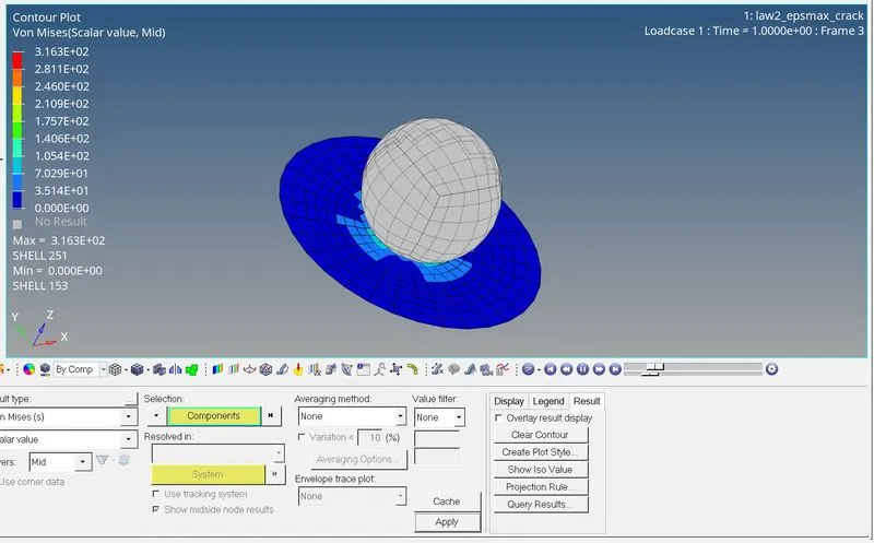
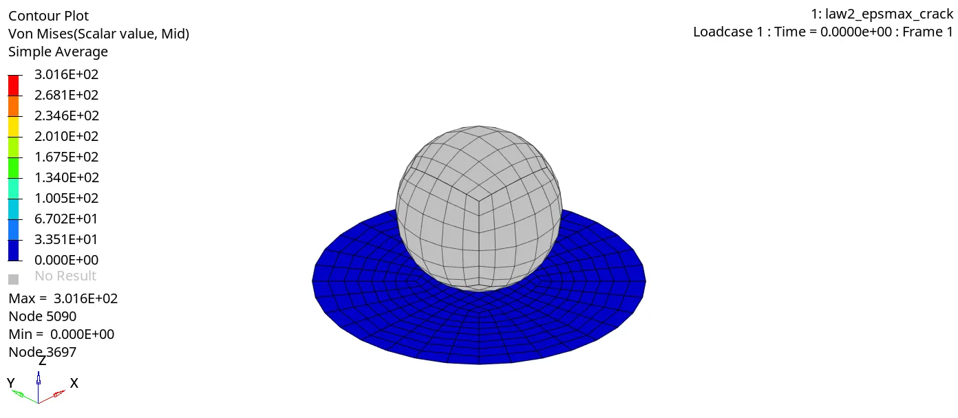
click on contour to apply von mises failure, and give average method as simple and click apply.

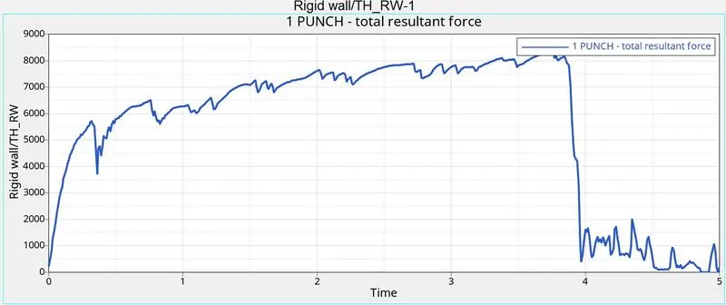
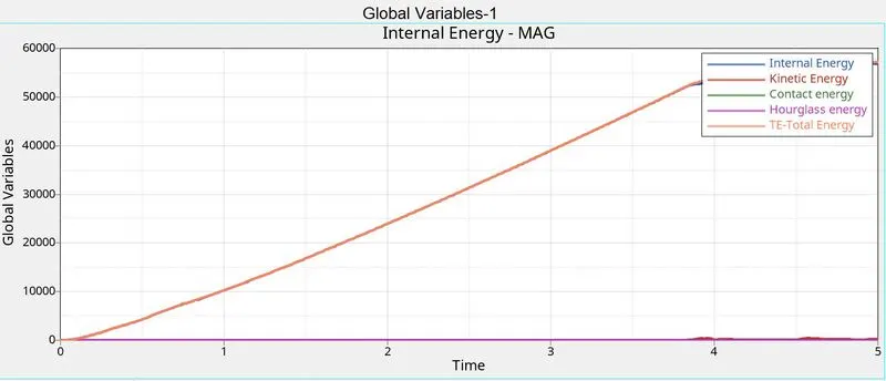
With the given results we have to plot all the energies in the hypergraph window. so at the 1st plot rigid wall forces and plot internal, contact, hourglass, total energy.

CASE 3

In this case delete the failure johnson card and run the simulation with no change.

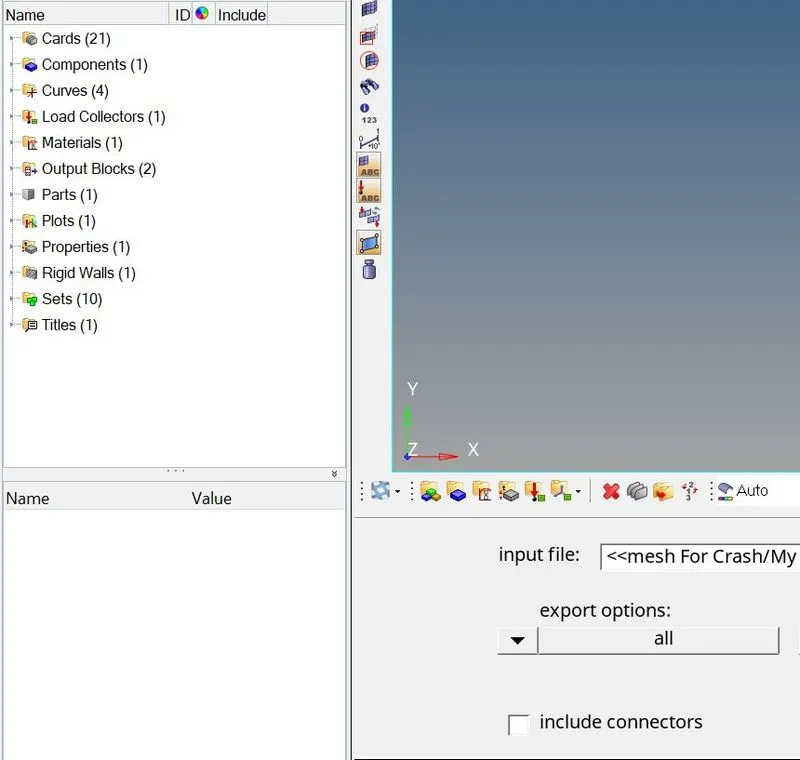
after the deletion run the simulation with new file named as law2_epsmax_nofail0000.rad and save as new folder.

After completion open the out file to examinate the results and energy error.

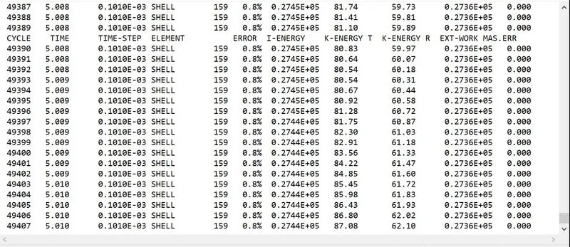
The results that are 49407 cycles, energy error=0.8%, internal energy=0.2744E, Kinetic energy=87.08, mass error=0.000. the energy error is almost zero.

Now open hyper view and import the h3d file and apply von mises analysis. This animation shows plate is breaking because of the elasto plastic material.

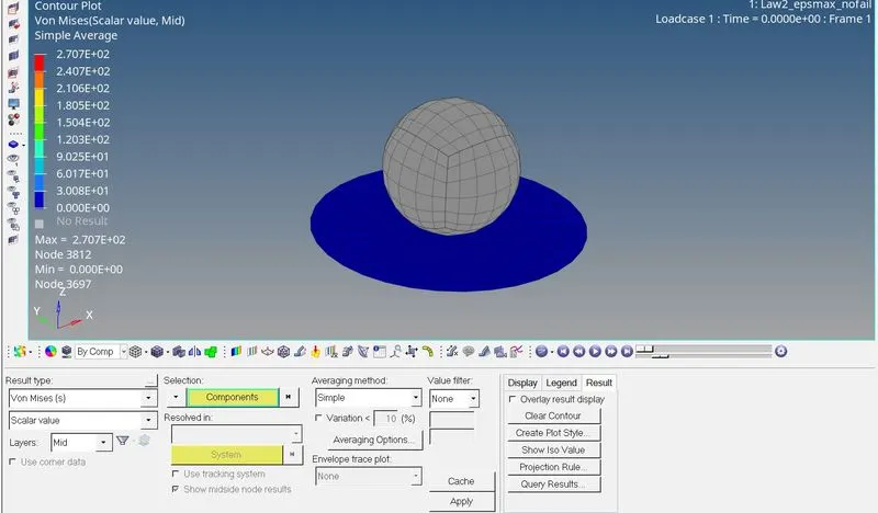
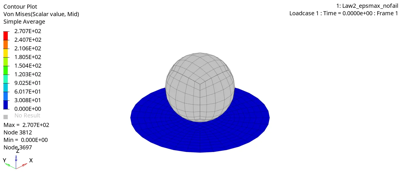
After completing the von mises analysis switch it to hypergraph 2d. Import t01 file in the data file option and plot rigid wall forces.

CASE 4

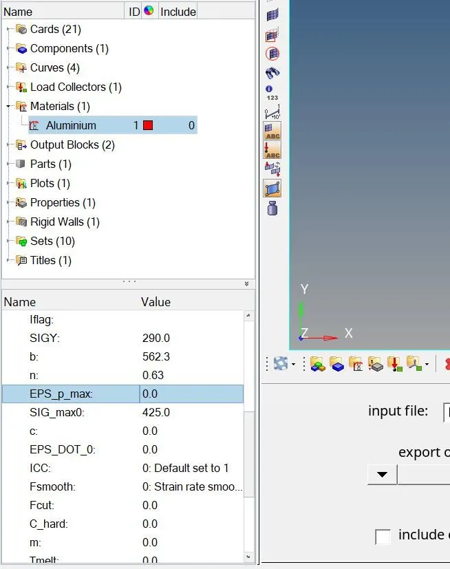
In this case deleting the epsmax(plastic strain)value and it becomes 0, and to check the results in this simulation. for that importing the last case starter file in the hypermesh and change the value to zero in the material card and start the simulation. like the last case save it in a seperate folder and save as law 2.

After the simulation open the 0001.out file to view the results.

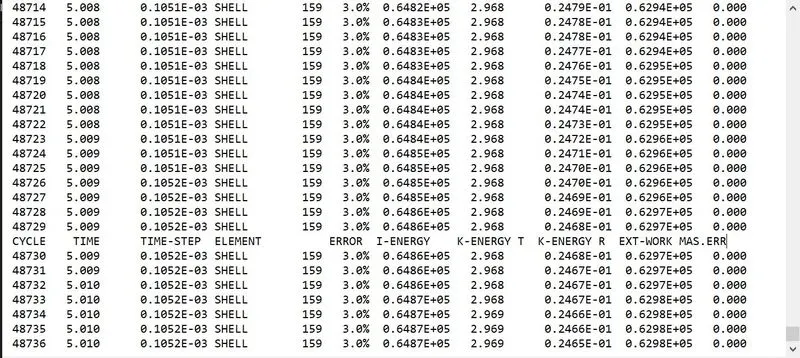
No of cycles=48736, Error=3.0%, Internal energy=0.6487E+05, Kinectic energy=2.969, Mass error=0.000.

the error of this case is high compared to other cases. we can talk about it in the end comparision.

Now import h3d file in the hyperview window to view the simulation.

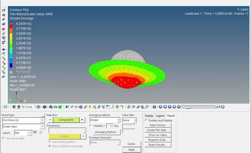
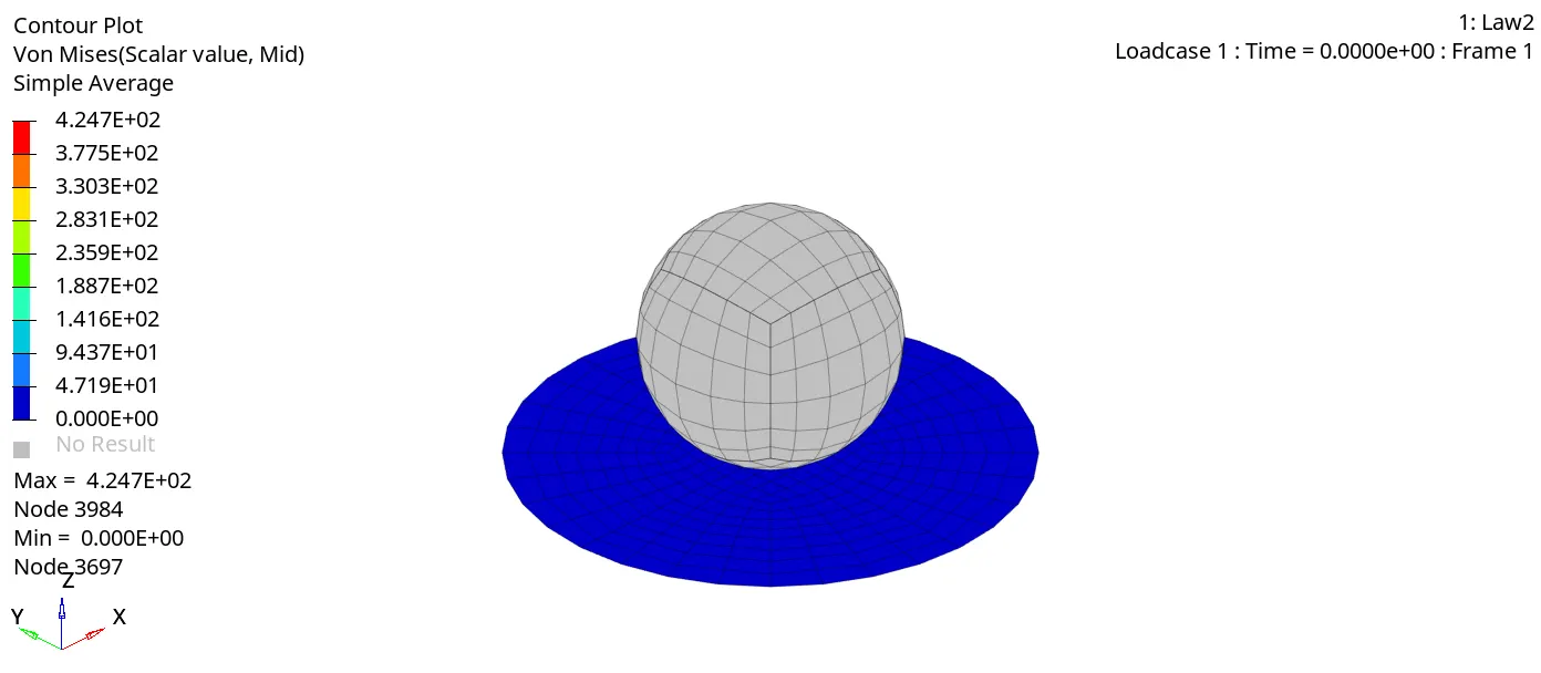
here elements are deleted but they strain itself to the higher value because of normal strain(ebsilon)=0.

Now import the t01 file in the hypergraph window. plot rigid forces in the seperate window.

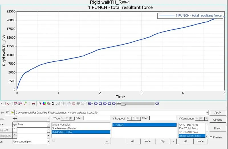
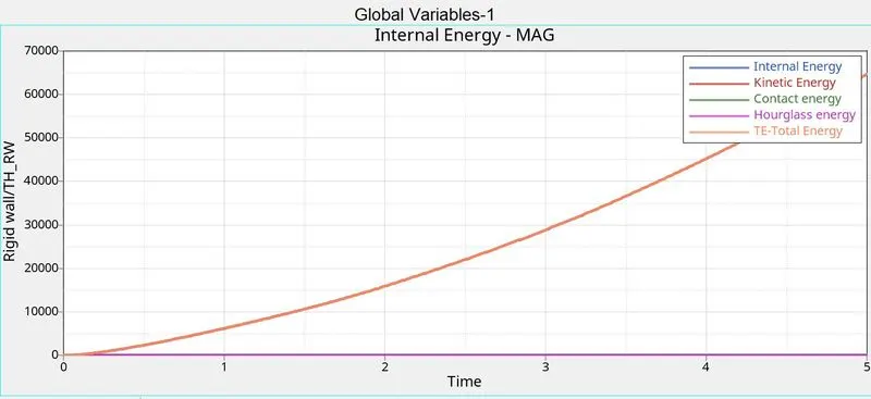
CASE 5

In this case import the failure johnson 0000.rad file run the simulation with the new name as law1_elastic_0000.rad. Here LAW1_ELAST should be changed & density`rho`, E(youngs modulus), Poisson's ratio`nu` can be changed with referece image.

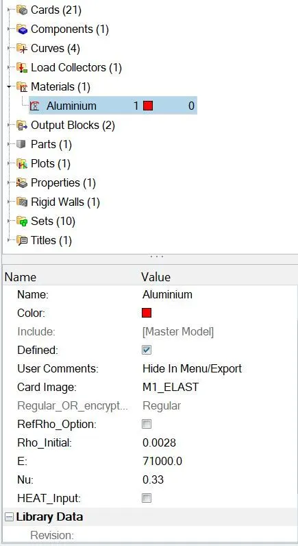
RUN the simulation and save it. open the 0001.out file and check the results.

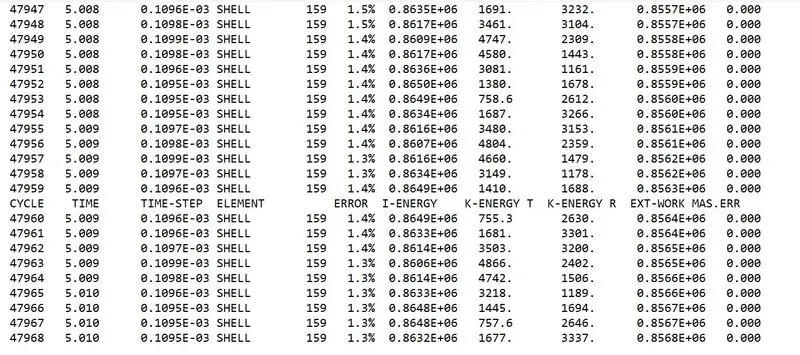
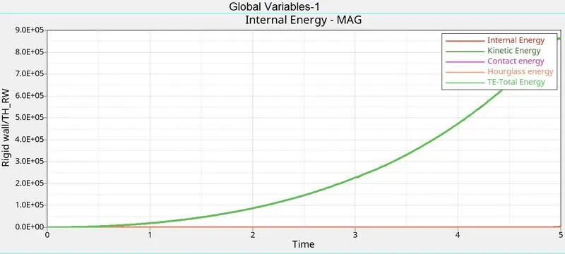
here no of cycles=47968, Error=1.3%, Internal energy=0.8632E+06, Kinetic Energy=1677.0, Mass error=0.000.

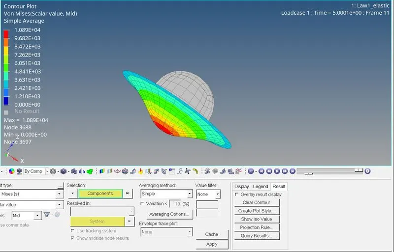
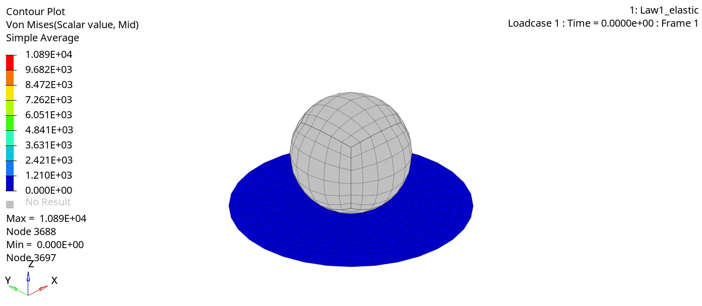
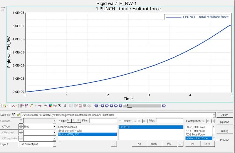
The applied law 1 elastic didnt lose the elements to break. it follows the isotropic elastic.

Now plot the rigid forces in hypergraph.

CASE 6

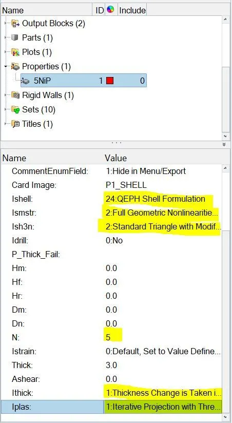
In this case import law 27_0000.rad file and change it recommended properties and run the simulation. IN prop card change it to Ishell=24, Ismstr=2, Ish3n=2, N=5, Ithick=1, Iplas=1.

Now run the simulation & save it in a new folder.

After the simulation open 0001.out file to view the results.

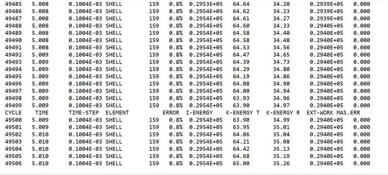
here the energy error is very close to 0, the error is 0.8%, and mass error is 0.

So we cana proceed with hyperview, Like the past import h3d file and enable contour for von mises to view the simulation.

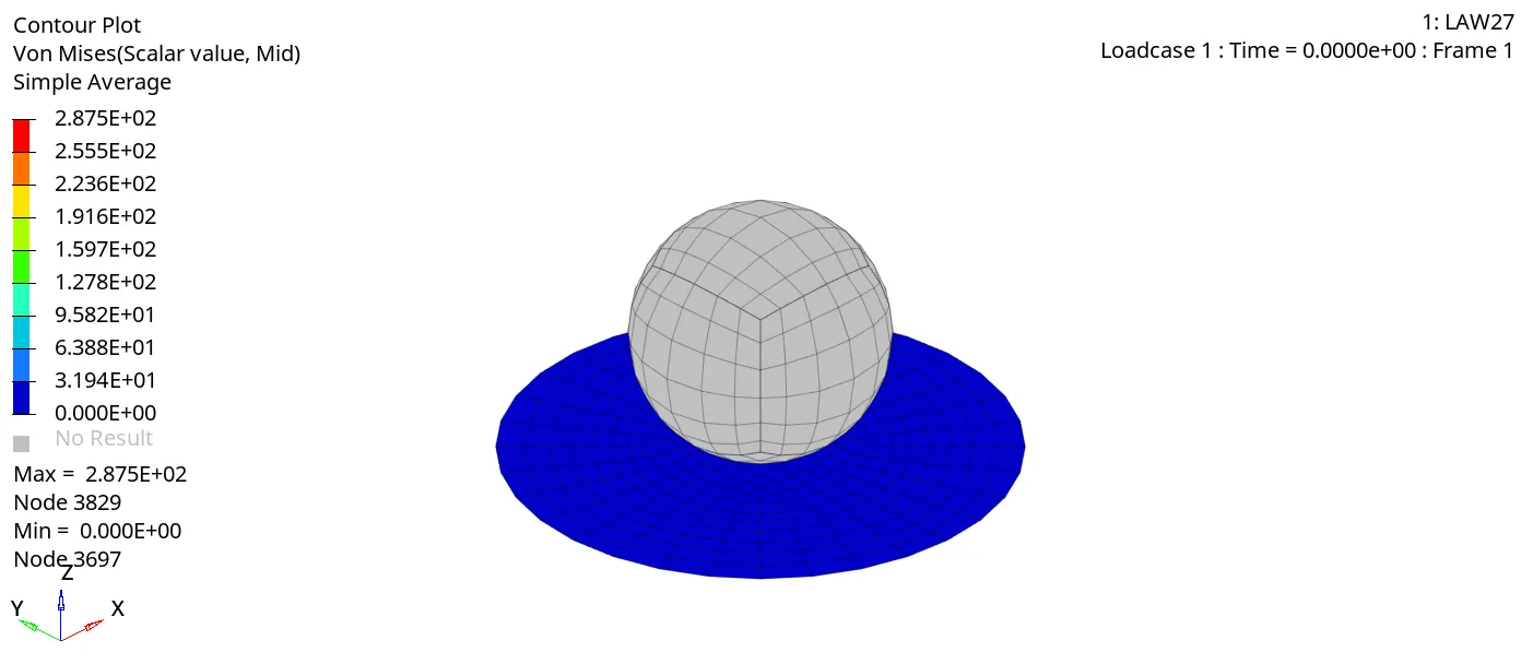
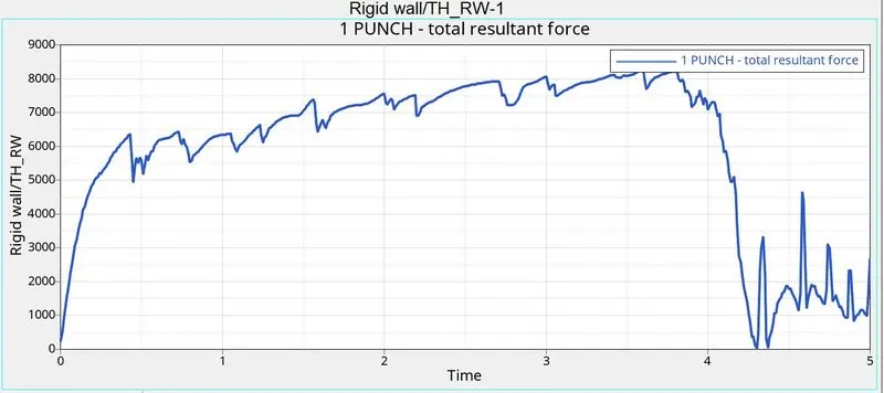
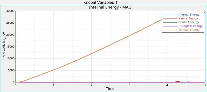
Now switch it to hypergraph. Import the t01 file and plot the rigid wall forces. Also plot the internal energy, contact energy, Hourglass energy, Kinetic energy, Total energy.

CASE 7

In this case import the same law27, change the card to law36 (Elasto plastic piecewise linear material). And the shell parameters in the property card is changedd to the recommended properties.

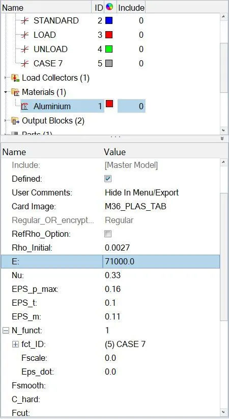
change the rho,E,nu and N function to define a curve. Create a new curve and name it as case7.

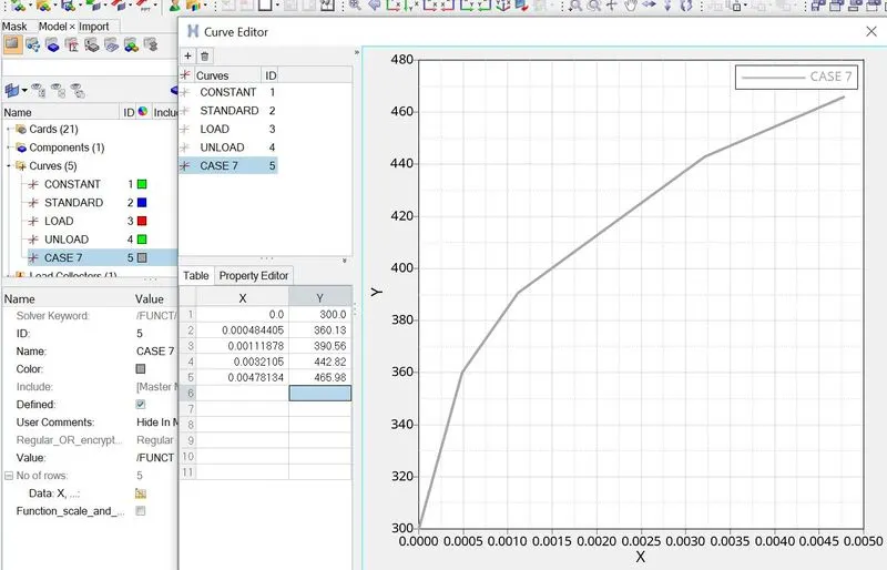
Use the curve coordinate values from card image from the video and plot a curve. Higher the curve the higher the strain rate. Then run the simulation and save it in a new folder.

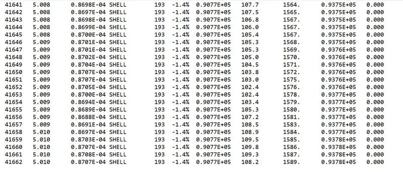
Open the 0001.out file to view the obtained results.

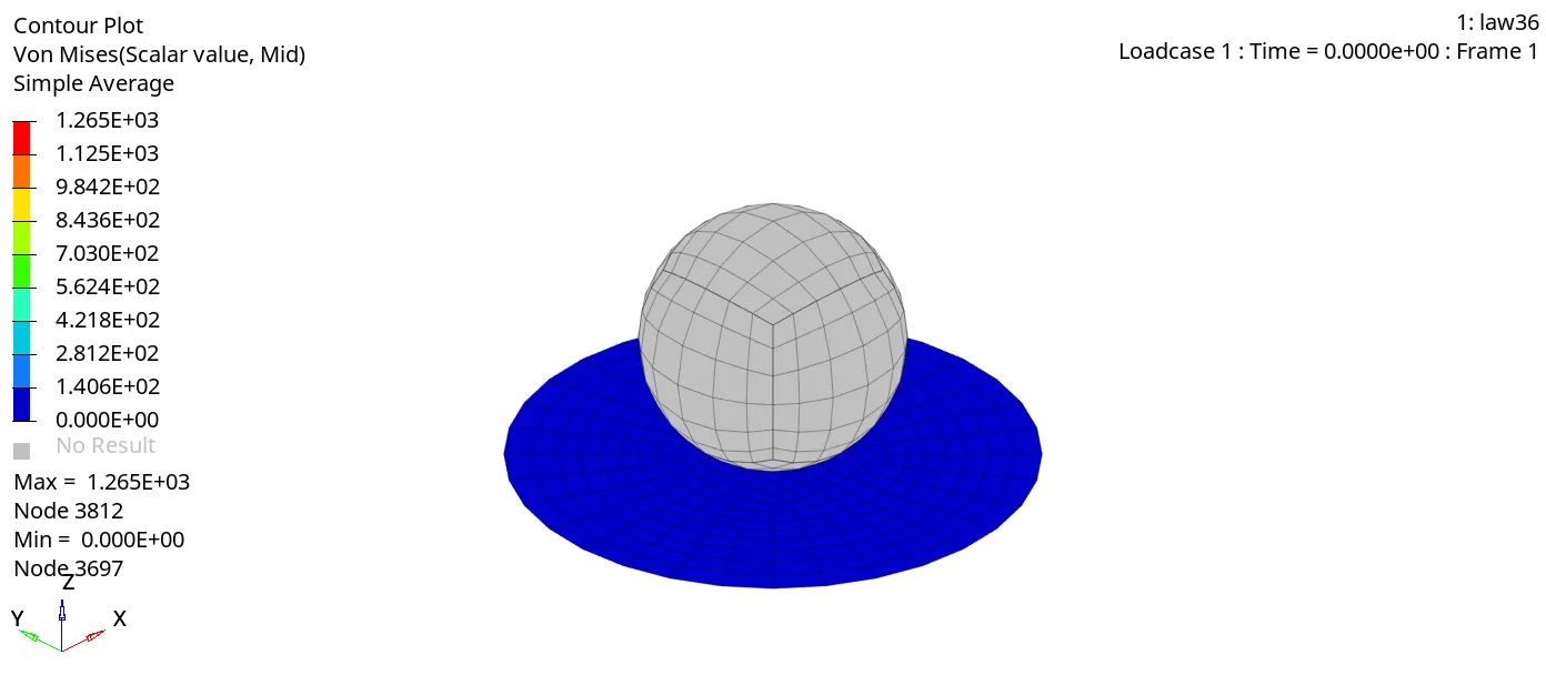
Now open the hyperview and import the h3d file and plot contour.

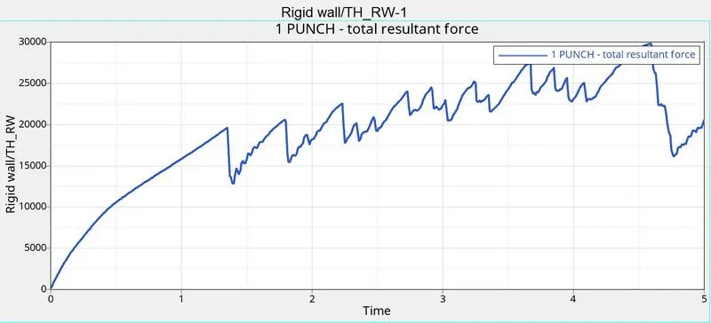
Plot rigid forces and global energies by importing the t01 file.

COMPARISONS

RESULTS/CASES	CASE 1	CASE 2	CASE 3	CASE 4	CASE 5	CASE 6	CASE 7
CYCLES	49379	49417	49407	48736	47968	49506	41662
ERROR	0.8%	2.2%	0.8%	3.0%	1.3%	0.8%	1.4%
I-ENERGY	0.2730E+05	0.5695E+05	0.2744E+05	0.6487E+05	0.8632E+06	0.2954E+05	0.9077E+05
K-ENERGY	67.81	236.6	87.08	2.969	1677.	65.00	108.2
EXT-WORK	0.2721E+05	0.5610E+05	0.2736E+05	0.6298E+05	0.8568E+06	0.2940E+05	0.9378E+05
MASS ERROR	0.000	0.000	0.000	0.000	0.000	0.000	0.000
ELEMENTS	deleted	performs elastic and deleted under higher strain because of values from failure card.	deleted	not deleted beacuse of default epsmax	not deleted because of elastic card property	deleted	deleted

• In the above all cases hourglass is nearly zero.
• In case 1,3,6,7 elements are completely deleted. elements undergo deformation and after deleting in the case 2.
• elements are not deleting because of higher elastic strain in the elastic card property(case5).
• Also in case4 plate undergo elastic because of deleting the plastic stain to zero.

CONCLUSION

In this assignment we learnt about the material cards, failure cards and types of energies based on simulation. here we have to use appropriate material laws for the component to get the better real time results which will match the prototype materials. In case 1,3,6 have very lesser error in the simulation,but the elements behaviour in the law 36 elasto plastic behavior. Hence we can conclude the law 36 and law 2 can be used for the scenarios.