Assignment 4-RADIOSS Material Laws Challenge

Assignment no 4

RADIOSS Material Law Challenge

 

Aim: To study the different material cards and their application in RADIOSS, and how to apply them in the RADIOSS

Objective:

Performing a simulation of sphere pressing on plate for different material laws and comparing the results. There will be 7 cases that we have to perform according to parameters and the material card given and then we have to compare the result via animation and plots, The file to be worked on are the FAILURE_JOHNSON_0000.rad and LAW27_0000.rad file, The following cases are

1. Law2 (File: FAILURE_JOHNSON_0000.rad – base simulation)
2. Law2 (File: FAILURE_JOHNSON_0000.rad) with Ifail_sh = 1, Dadv = 1 and Ifxem = 1
3. Law2 (File: FAILURE_JOHNSN_0000.rad) with Fail_JOHNSON card deleted
4. Law2 (File: starter file for case 3) with EPS_P_max value deleted
5. Law1 (File: FAILURE_JOHNSON _0000.rad) with Fail_JOHNSON card deleted and values of E, nu, rho value need to be defined
6. Law27 (File: LAW_27_0000.rad) with recommended shell properties
7. Law 36 (File: Law27_0000.rad) with recommended shell property and given reference curve

These are the following cases that we need to perform and comparing the results

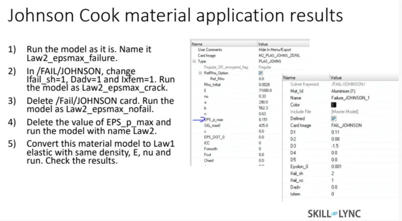
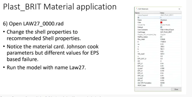
The following Parameters we need to follow to compare the result among the different cases

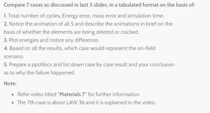
Given by the Technical Support team

Theory:

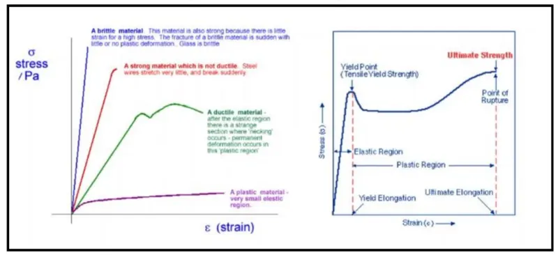
Source: Skill-Lync

The fig. 2 represent the Elasto-Plastic Plot

 

• The accuracy of the simulation depends upon the material chosen.
• Choosing the right material and providing the reliable material data in performing a simulation is very easy.
• RADIOSS have multiple material property and wide variety of material like concrete, foam rubber, composites etc.

Some of the commercial used material laws are

 

1. Law1: Elastic (Isotropic elasticity)
2. Law2: JOHNSON_COOK (Isotropic elastoplastic)
3. Law27: Elastic-Plastic Brittle
4. Law36: Elastic-Plastic Tabulated
5. Law42: Ogden (Visco-hyper-elastic)
6. Law70: Fam

Isotropic Elasticity (Law1):

• Isotropic means material will have same material properties in all three directions. Under isotropic elasticity RADIOSS provide two types of elasticity,

1. Linear Elastic: Law1 Elastic
2. Hyper-elastic: Law69 Tabulated hyper-elastic, Law82 Ogden

• The RADIOSS elasticity law follows Hooks law of elasticity I.e. linear relationship between Stress and Strain.
• It is available for truss, beam, Shell and solid elements
• The material stiffness is determined by Young’s modulus of Elasticity(E) and Poisons ration(n).
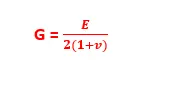
• The Shear Modulus G is calculated by

 Limitation:

 

• Elastic material can’t be used for large deformation cases such as blow molding etc.
• In case of large deformation, Law2 Johnson-cook material with high yield can be used

 

Isotropic Elastoplastic

• RADIOSS provides various types of elasto-plastic material laws, it has all material models based on Von-misses hardening without damage, von-misses with ductile damage, von-misses with visco-plastic flow
• Here we are going to look at Johnson-cook/JOHNS and tabulated piece-wise linear/PLAS_TAB

 

(PLAS_JOHNS) johnson-cook material – Law2

• This Law represent isotropic elasto-plastic material using the Johnson cook material model
• The model express stresses as function of strain, strain rate, Temperature
• In a material card, we have option called EPS_max which is nothing but Plastic stain at failure. Failure of element happens, when one integration point reaches EPS_max
• No if failure is based on EPS_max there can be instances where EPS_max gives out unrealistic result. To avoid this, we have option called /FAIL/JOHN.
• /FAIL/JOHN card provides the user with more control over the failure of Johnson-cook strain

Law36 – PLAS-TAB Elastic plastic piecewise linear material

• The Law 36 material law helps in modelling isotropic elasto-plastic material using user defined function for the work hardening portion of the stress-strain curve for different strain rates
• The curve defined is nothing but the stress-strain curve after the yield point, The yield point is set to 0 strain.
• The material law is available for both brick and shell elements.
• If work hardening portion is defined by user then, its elastic portion is taken from the inputted Young’s modulus and poisons ratio
• Any number of stress-strain curves can be defined
• The important part is that strain rate curve must not intersect each other

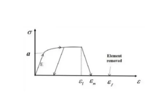
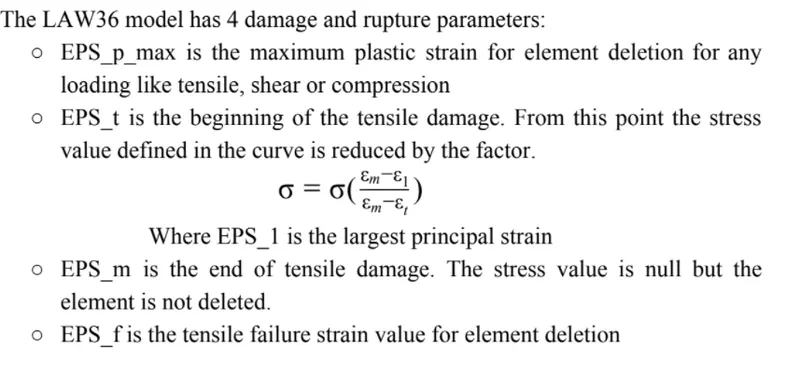
• The plastic strain curve is start with 0
• The user has option to input yield stress with respect to pressure using fct_Idp

We also have other laws that is used for different applications and conditions

Test run on the model with increasing the Simulation time 

PROCEDURE:

 Case 1:

• Open Hyper-mesh, go to import > Solver-deck option > Browse file > Import. The FAILURE_JOHNSON_0000.rad file is imported
• After importing the file first, we need to check-out the unit system that we need to follow, for that go to cards > Begins card

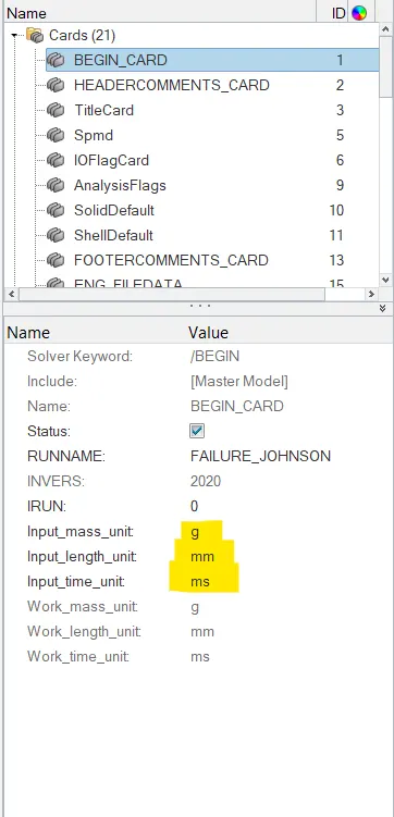
• Now in case1 we have to run the simulation as it is, but before that we have to check whether parameters related to element is correct or not

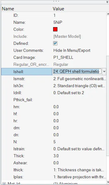
Checking of Shell element formulation and their related parameters

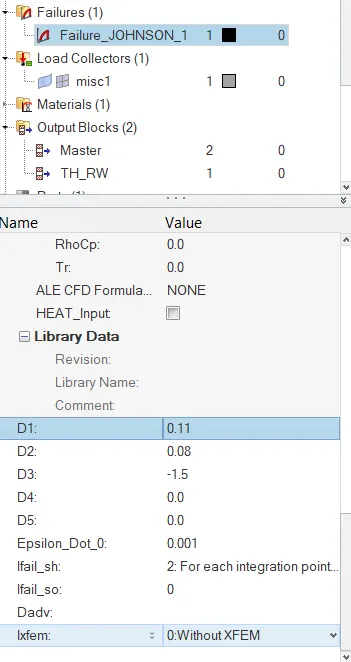
Default values of properties, Material and Failure cards

• To run the simulation, go to Analysis >> RADIOSS, we have to save the file as Law2_epsmax_failure_0000.rad file as per given instruction, after that click the include connector box and type as -nt 3, the -nt 3 means the number of cores, you want to use to run the simulation, Here, we have only 3 cores so we choose -nt 3. whereas, nt means “numbers of threads”, After that click on RADIOSS to run the simulation.

• When solver will show your Job is completed, note the number of cycle it taken and the elapsed time which is nothing but time taken to solve the simulation

Total no cycle = 49380

Elapsed time = 54.11s

 

• Now after that we have to check the energy error and mass error in our simulation to validate the simulation result. To check the error, open the out file in Notepad.

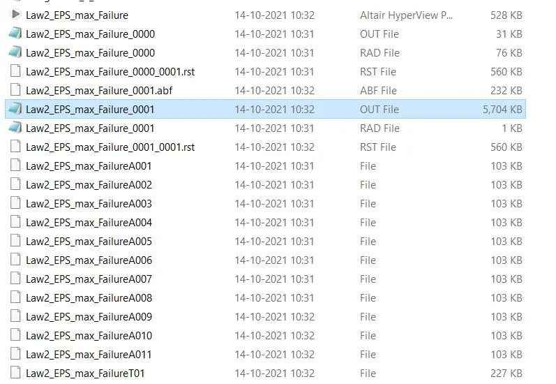
No of Files generated by solver that contains the results

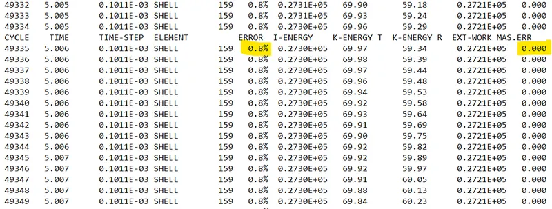
Engine output file for case 1

Here we have no mass error and the Energy is 0.8% which is in acceptable range.

• After that we need to visualize it. For that we need to switch to the Hyper-view utility, in hyper-view we need to import the h3d file that was generated during solving. Now to display the result we need to select the result plot we required, here we check von-misses contour by selecting Global variable as Von-misses, and here we use averaging method as simple to visualize the result.

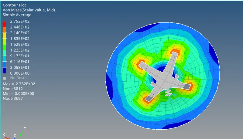
Von-Misses contour plot

• Now to plot the graph we need to switch to the Hypergraph 2D. we can switch to it using the same client sector option in toolbar, also in single window we can split it into number of windows, where we can plot the different plots. To plot the graph, we required the T01 file to upload to see the graphs. This file is available in same directory where we have .out files, h3d files, here we can plot different graphs like Rigid wall forces, Internal energy, Kinetic energy, Hourglass energy, Total energy to compare and visualize the result.

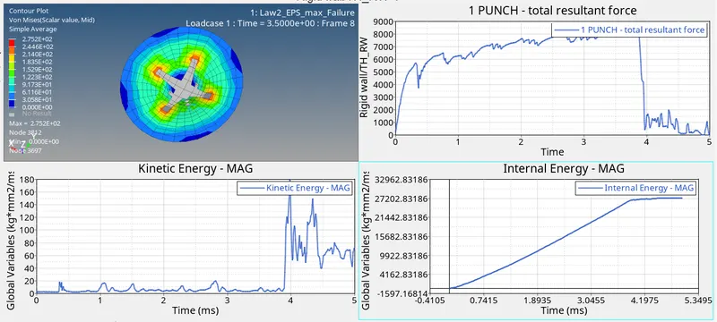
Rigid wall force / Internal energy and Kinetic energy

Observation:

• Here we have FAIL_JOHNSON card to define the failure criteria. In this card we have EPS_P_max value is defined with Ixfem value as 0. EPS_P_max is nothing but plastic strain at failure. This means that the element is deleted as it reaches to EPS_P_max threshold, because our Ixfem value is zero, it means our element is directly deleted instead of cracking into smaller element. This is what you can observed in the simulation, near center of the plate the element is reached to the EPS_P_max value and it is deleted, so the crack is intiated from the center and it go away from center, and element is deleting as it reaches to EPS_P_max value.

• Internal energy forces as well as Rigid-wall forces are the reactions to the force generated by the sphere on sheet. As you see from the graph Rigid wall forces increase at initial level, but due to element deletion there is fluctuation in the force, and at 4ms large chunks of element got deleted because it reaches to the threshold value of EPS_P_max, due to this Rigid wall force drops immediately, because there is no resistance left for the ball, or in other way we can say that there is not many element that opposes the force Spherical ball, Most of the element in its path have been deleted at that point, so due to this rigid-wall force drops.

• As you see the Kinetic energy also fluctuate as element is deleted, from the graph it is seen that as element deleted there is fall in the rigid wall force ad increment in the kinetic energy. As you see at 4ms most of the element are got deleted, due to this there is not many elements left that opposes the sphere, due to this there is increase in its kinetic energy.

Note: Area under the curve is energy absorbed while deleting the element, because the elements as absorbed so much energy, now it is deleted, so there is no way for us to get energy back.

Case2:

In case 2 we have to do some changes in the FAILURE_JOHNSON_0000.rad via the solver deck, to do changes in failure card, we can access this card in the model tab, we have to change or set the value of (Ifail_sh = 1, Dadv = 1 IXFem = 1) in the failure card.

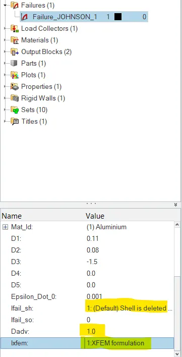
Changes in the Failure card

Ifail =1, which determine the shell element failure method, so there are two way in which we can see the element failing, on is simply deleting of the element, or in some cases cracking is occurring in the element according to the material properties.

Ixfem = 1, from this option we can change or switch from element deletion to element cracking, when Ixfem = 1 the element is cracked when it reaches to threshold value, also due to the element cracking more energy is dissipated during the simulation.

Without Ixfem treatment our elements got deleted whenever you should seen a crack, since element are going to crack it gives more realistic results

Dadv: It gets activated when we have taken Ixfem = 1, for that we have to take Dadv = 1 which is nothing but the criterion for the crack advancement.

• After defining all these parameters run the analysis in same manner and save the file as Law2_epsmax_crack_0000.rad with include connectors ticked and -nt 3 typed in the option box to activate the number of cores to solve the problem.

• After the solver complete the analysis note the Total number of cycles, Run time or Elapsed time.

In case 2 the Total number of cycles = 49217, Elapsed time = 68.61s

• Now after that we have to check the energy error and mass error in our simulation to validate the simulation result. To check the error, open the out file in Notepad.

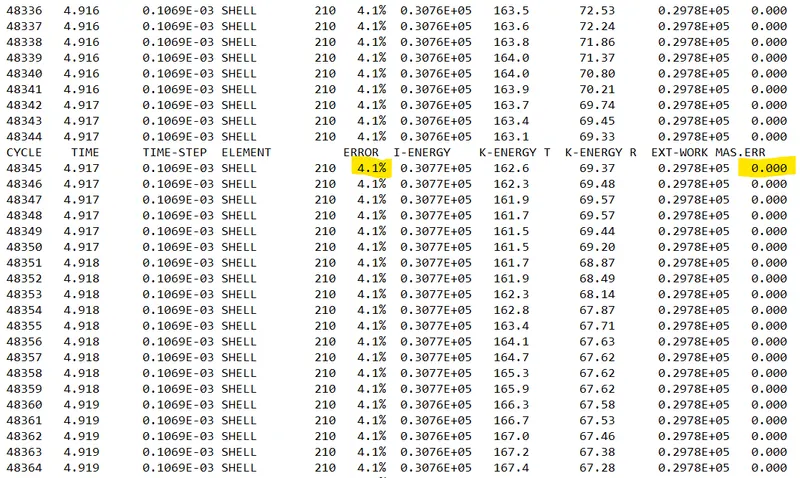
Engine output file for case 2

 Here we have Energy error = 4.1% Mass error = 0.00%, which is under acceptable range, but still near to the threshold value of Energy error.

• Again, to visualize or to check the result, we need to switch to the Hyper-view utility, in hyper-view we need to import the h3d file that was generated during solving. Now to display the result we need to select the result plot we required, here we check von-misses contour by selecting Global variable as Von-misses, and here we use averaging method as simple to visualize the result.

• Now to plot the graph we need to switch to the Hypergraph 2D. we can switch to it using the same client sector option in toolbar, also in single window we can split it into number of windows, where we can plot the different plots. To plot the graph, we required the T01 file to upload to see the graphs. This file is available in same directory where we have .out files, h3d files, here we can plot different graphs like Rigid wall forces, Internal energy, Kinetic energy, Hourglass energy, Total energy to compare and visualize the result.

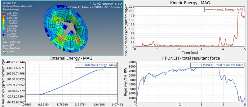
Rigid wall Force / Kinetic energy / Internal energy

Observations:

 

• Here we use the Ifail_sh, Dadv, Ixfem as a part of Johnson failure card, as we defined Ixfem, now instead of deleting the element when it reaches to max plastic strain, our elements got cracked into smaller elements and dissipated more energy as compared to previous case. but it shows the stress value slightly more than the previous one.

• Here as you see the graph, Rigid wall force is start increasing from 0 when the sphere starts to collide with the plate, with time the rigid-wall force start declines and kinetic energy of the sphere start increasing because of not enough elements that opposes or restrict the sphere. Due to this you can see the fall in Rigid-wall force and increment in the Kinetic energy of the sphere.

Note: For Ixfem to use, your material model needs to be very accurate, also the way Ixfem work, it dissipates more energy, because of that for smaller crack propagation (local deformation) Ixfem is a good method, but if you want to see how a crack is propagating along a longer distance then in that case Ifxem is not a good method to use.

Case3:

In this case again we use the same starter input file named as FAILURE_JOHNSON_0000.rad file, but here we have to delete the Johnson failure card.

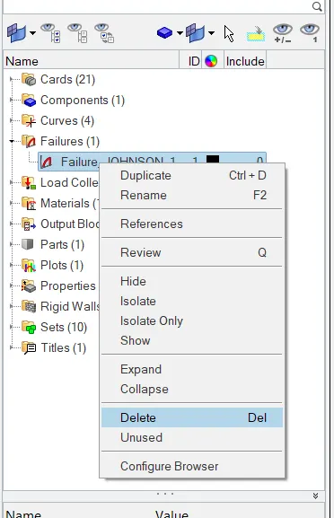
Deleting Failure Jonson card

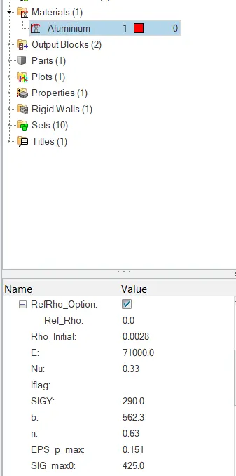
But still, we have EPS_P_max failure criteria for the element.

• After deleting the material card, we can run the analysis in same manner as mentioned above.

In this case

Total number of cycles = 49408 and Elapsed time = 55.63s

Mass error and Energy error

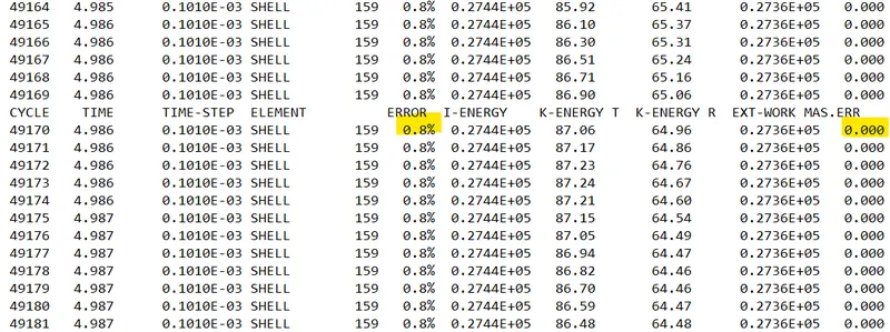
Energy error = 0.8% and mass error = 0.00% (Energy error is close to 0 which is in acceptable range)

 

• To check the result, again we need to open h3d file in Hyper-view, and plots the contour according to ourself. Here we plot the Von-Misses contour to check the result.

• Now to plot the graph we need to switch to the Hypergraph 2D, and here we need to import the T01 file to see the various energy plots.

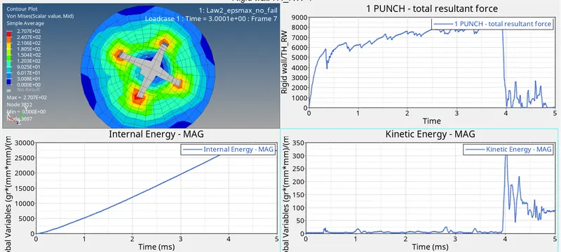
Rigid-Wall force / Internal Energy / kinetic Energy plots

Observations:

• With the Fail/Johnson card deleted in this case, we have EPS_P_max factor for element deletion, so when element reaches to 15% of plastic strain it deletes the element, Here element is deleted much more faster as compare to case2 where element is cracked into smaller element instead of deleting the element.

• There is linear increase in the Internal energy until a bulk of element is deleted from the model, so the energy absorbed by the element got wasted due to element deletion.

• Due to this there is sudden drop in the rigid wall force (and increase in K.E) at the same time step, because the element that were in contact with sphere during collision is deleted. The Rigid wall force which is basically the opposing force generated by the metal sheet against sphere. So due to element deletion there is lot of fluctuation you can observe in the Rigid wall force and Kinetic energy plot.

Case 4:

Here we have to delete the value of EPS_P_max from the previous case file and run the simulation and named it as Law2

• Import the case 3 starter file law2_epsmax_nofail_0000.rad, In this file we have to delete the value of EPS_P_max or we can say that we have to set this value to zero.

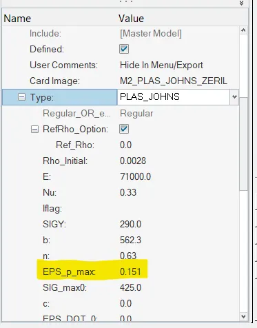
Set EPS_P_max = 0

• After that we can run the analysis for solving and save file as Law2_0000.rad.

we can run the analysis in same manner as mentioned above.

In this case

Total number of cycles = 49304, Elapsed time = 58.22s

 

 

Mass error and Energy error

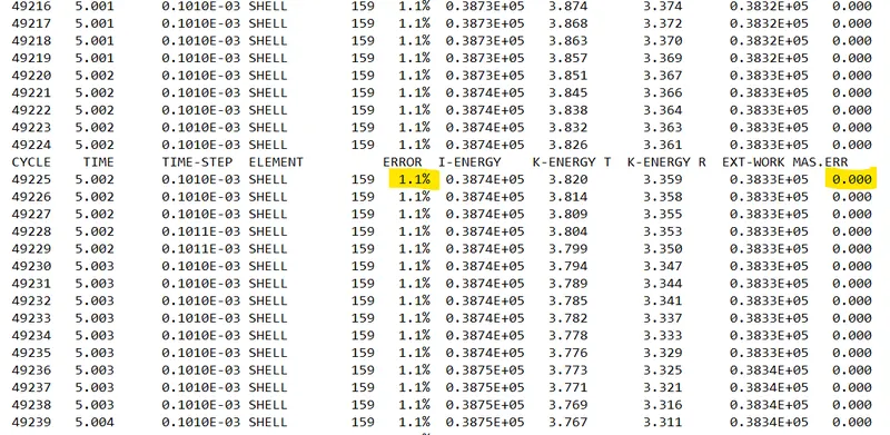
Here the Mass error is 0 and Energy error = 1.1% which is in acceptable range

 

• To check the result, again we need to open h3d file in Hyper-view, and plots the contour according to ourself. Here we plot the Von-Misses contour to check the result.

• Now to plot the graph we need to switch to the Hypergraph 2D, and here we need to import the T01 file to see the various energy plots.

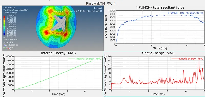
Rigid-Wall Force/ Internal Energy / kinetic energy plots

 

Observations:

• Here metal sheet is able to withstand large amount of strain and avoid element deletion due to the fact that the value EPS_P_max is set to 0, due to this RADIOSS set it to default value of 10^30, also here the Johnson fail card also has been deleted. But still here the element is deleting because there is one more threshold value of sigma_max, if element is crossing them then it got deleted. So at regular interval of time, we see the fluctuation in Kinetic energy due to element deletion. Also, one more thing to notice that the Kinetic energy generated in this case is almost negligible as compared to other case.

 Case 5:

Converting the model to Law1 Elastic with same density, Young’s-modulus(E), Poisons ratio (nu)

• In this case firstly import the starter file FAILURE_JOHNSON_0000.rad, after that go to materials > Aluminum and change the card image to Law1 Elastic (M1_ELAST)
• Also set the value of Rho initial, E, nu as follow

Rho for aluminum 0.00271

Young’s modulus for Aluminum (E) = 71000

Poisons ratio (nu) = 0.33

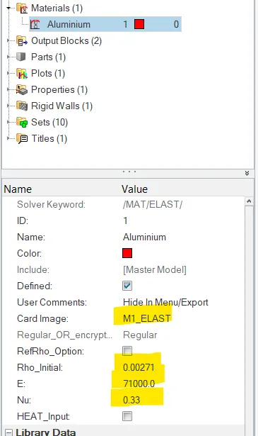
Material changed to Law 1 Elastic

• Now solve the file by clicking on RADIOSS and save the file as Law1_0000.rad, after solver solve the file completed note the Total number of cycle and Elapsed time

Total number of cycles = 48418

Elapsed time = 52.59 s

• After that we have to check the energy error and mass error

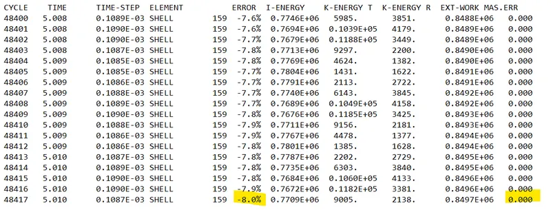
The mass error is negligible and almost 0 whereas the Energy error is -8.0% which is in acceptable range.

 

• To check the result, again we need to open h3d file in Hyper-view, and plots the contour according to ourself. Here we plot the Von-Misses contour to check the result.

• Now to plot the graph we need to switch to the Hypergraph 2D, and here we need to import the T01 file to see the various energy plots.

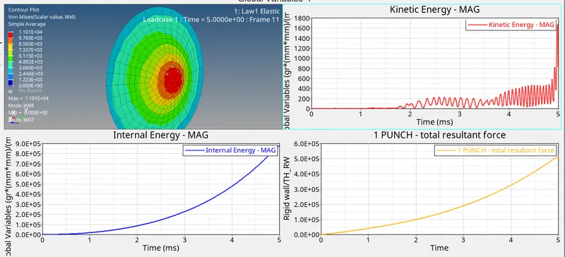
Rigid-Wall force / Internal Energy / Kinetic Energy

 

Observations:

• In this case the plate is defined with M1 Elastic, this means that plate behaves in completely elastic manner, means when load is removed it come back to the original shape, so there is no plastic deformation which result in linear deformation.
• As you see here due M1_Elast card the metal sheet is absorb the large amount of energy of impact, The above model we use it is for the purely elastic material, this explain the why element is not going to delete or rupture, due to this it behaves like a membrane which absorb large amount of energy, due to this large amount stress is observed on the metal sheet about 11010Mpa, which is large value as compared to Law2
• The Kinetic energy gradually increases as plate is stretched to maximum limit for the applied load, also due to the elastic nature the Internal Energy and Rigid-Wall force both increasing exponentially. Both Internal energy and Rigid wall forces increases due to the absorption of kinetic energy from the impacting sphere and down once the plate return to original shape.

Case 6:

• In this case import the starter file as LAW27_0000.rad file, we need to check the properties and shell element formulation and their parameters in this case. For that go to Properties > 5Nip. Here, we have to set the various parameter as follow

I_shell = 24 (QEPH), I_smstr = 2, I_sh3n = 2, I_thick =1, I_plas = 1

• After checking all the properties, we can now solve it by clicking on the RADIOSS button and save the file as Law27_0000.rad

 

• When solver completely solve the file, note the Total number of cycles and Elapsed time

 Total number of cycles = 49508, Elapsed time = 56.64s

• After that we have to check the energy error and mass error

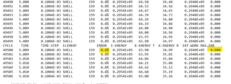
Mass error is 0 whereas the Energy error is 0.8% which is in acceptable range

 

• To check the result, again we need to open h3d file in Hyper-view, and plots the contour according to ourself. Here we plot the Von-Misses contour to check the result.

• Now to plot the graph we need to switch to the Hypergraph 2D, and here we need to import the T01 file to see the various energy plots.

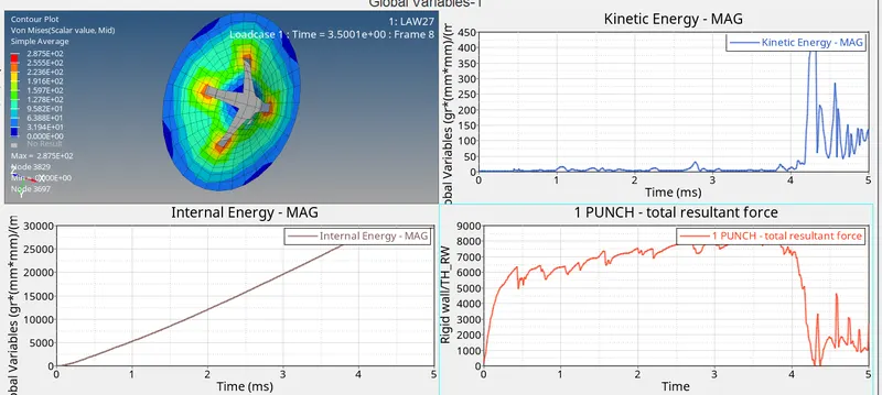
Rigid-Wall force / Internal Energy / Kinetic energy

 

Observations:

• In this case we using M27_PLAS_BRIT material card which combines an isotropic elasto-plastic Johnson-cook material model with an orthotropic brittle failure model.
• If we compare it with case 1 what we observe that the stress value is more in this case as compared to case1, this is because here material behave in brittle manner and don’t able to dissipate large amount of energy, due to this material will fail in brittle manner, and at 4ms large amount of chunk of element got deleted due to this there is no resistive force or reaction force experienced by the sphere, so due to this Rigid wall forces which is actually a reaction force that is applied by metal sheet to sphere starts decreasing with element deletion, also with element deletion Kinetic energy starts increasing.

Case7:

• In this case import the LAW27_0000.rad again, we will edit some parameters in this case
• Go to the model tab and here we shall be creating a new curve as per the instruction, to create the curve, go to curve in model browser and then right click to create the curve, here we have to define the x and Y values to create the curve, also we define scale factor F= 1 because our unit is matching with unit used by the solver.
• Before that we deleting the Material-card and change it with the M36_PLAS_TAB (Law 36)
• As we know this law models an isotropic elasto-plastic material using the user defined function for work hardening portion of stress strain curve. Here also we define the work hardening portion of the curve for aluminum material.

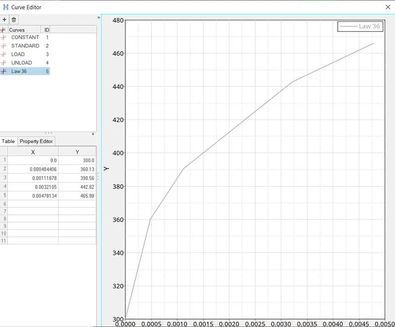
Creating a work-Hardening curve for Aluminum material (Lab Data at a particular strain rate)

• After that we have to define the N-funct = 1 and here we need to define the curve with Fscale = 1 whereas N_funct is the number of function which can be between 1 to 100 depending upon the different application, from this function we can define number of work hardening curves for the material at different strain rate.

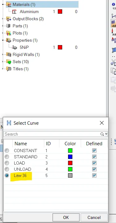
Defining the work hardening curve at a particular strain rate

• After defining all the parameters, now our solver can start to solve the file, once the solver will solve the file completely note the Total number of cycles and Elapsed time

Total number of cycles = 41664

Elapsed time = 47.72s

We also need to check the mass error and Energy error

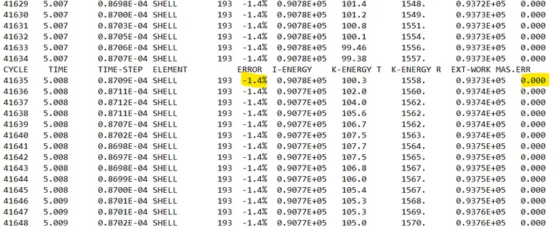
Mass error is 0 where ae Energy error = -1.4% which is in acceptable range

• To check the result, again we need to open h3d file in Hyper-view, and plots the contour according to ourself. Here we plot the Von-Misses contour to check the result.

• Now to plot the graph we need to switch to the Hypergraph 2D, and here we need to import the T01 file to see the various energy plots.

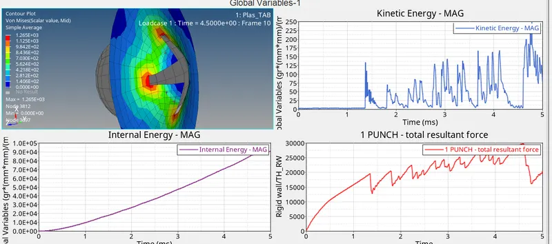
Rigid-Wall force / Internal Energy / Kinetic energy

 

Observations:

• Here we are using PLAS_TAB card where we define the Work hardening curve at particular strain rate based on the LAB data, here as you see there is lot of fluctuation in rigid wall forces and Kinetic energy, because element is deleted in continue manner once the element reaches to EPS_P_max , here the max stress we got is more than the case 2, but we can’t compare these results directly because we don’t know at what strain rate this impact has been done. The spikes in up and down of rigid-wall force and Kinetic energy is due to element deletion.

The Result of 7 Cases as Follow

Case	Material law	Simulation name	Energy error (%)	Simulation time (s)	Number of cycles	Maximum stress value (MPa)	Element condition under high stress
1.	Law2 (Johnson-cook material model)	Eps-max_failure	0.8	53.11	49380	275.2	Deleted
2.	Law2 (Johnson-cook model)	EPS_max_failure_crack	4.1	68.61	49287	295.1	Element undergo crack formation
3.	Law2 (Johnson-cook model)	EPS-max_nofail	0.8	59.63	49408	270.7	Deleted
4.	Law 2 (Johnson cook model)	Law 2	1.1	58.22	49304	245.1	Can’t be deleted due to the absence of Failure card and high value of sigma max
5.	Law1 (linear elastic material)	Law 1	-8	52.53	49418	11010	Can’t deleted due to elastic property card
6.	Law 27 (Brittle failure model)	Law 27	0.8	56.64	49508	287.5	Deleted
7.	Law 36  (Elasto-plastic model, Tabulated plastic)	Law 36	-1.4	47.72	41664	1265	Deleted

Learning Outcomes

 

• Understanding about different type of material cards
• Understanding about the failure cards
• Understanding about how the different cards and their parameters effect the result.

Conclusion

• Selecting a correct material model plays a very important role in the simulation
• The accuracy of the simulation depends upon the material chosen.
• Choosing the right material and providing the reliable material data in performing a simulation is very easy.
• RADIOSS have multiple material property and wide variety of material like concrete, foam rubber, composites etc.

Law1 is used to model purely elastic material or material that remains in the elastic range

Law2:  This law model isotropic elasto-plastic behavior. In this law the material behaves as linear elastic when equivalent stress is lower than the yield stress and also it capture plasticity and also with Failure card we can able to capture the failure as well

Law 27 is used for brittle material

Law 36: This law model elasto-plastic behavior of isotropic material with user defined function, means the work hardening portion of the curve has to be defined by the Lab result, we can put different work-hardening curves at different strain rates, and the elastic portion of the curve is simply defined by E, nu, Rho of the material. so the result we got near to the actual result. So, if we have Lab result then it is better to use this material model.