Assignment 4-RADIOSS Material Laws Challenge
MATERIAL LAWS CHALLENGE
Crashworthiness analysis using RADIOSS and Hypermesh- Assignment-4
AIM:
To run crash analysis on the given model by applying different materials laws available in Radioss and post-process the results
Objective –Run the given Models in Radioss as per the required parameters and compare them using the plots and animations.
- Given model – impact of a rigid ball on sheet of metal, for all these cases the material laws are changed for the sheet.
- Case 1 – Law 2 with EPS Max Failure and Failure Johnson card
- Case 2 - Law 2 with EPS Max Failure and Ifail =1, Dadv =1 and Ixfem = 1 (crack)
- Case 3 – Law 2 with deleted Fail Johnson card
- Case 4 – Law 2 with deleted Fail Johnson and EPS Max Failure
- Case 5 - Law 1 with density, E, nu
- Case 6 – Law 27 with EPS based Failure
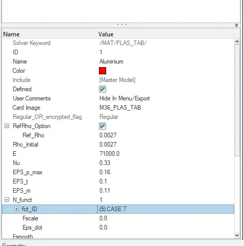
- Case 7 – Law 36 with Strain rates curve
- Law 1: Elastic (Isotropic Elasticity)
- Law 2: Johnson-cook (Isotropic Elasto-plastic)
- Law 27: Elastic-plastic brittle
- Law 36: Elastic-plastic tabulated
- Law 42: Ogden (visco hyperelastic)
- Law 70: Foam
PROCEDURE:
Case 1:
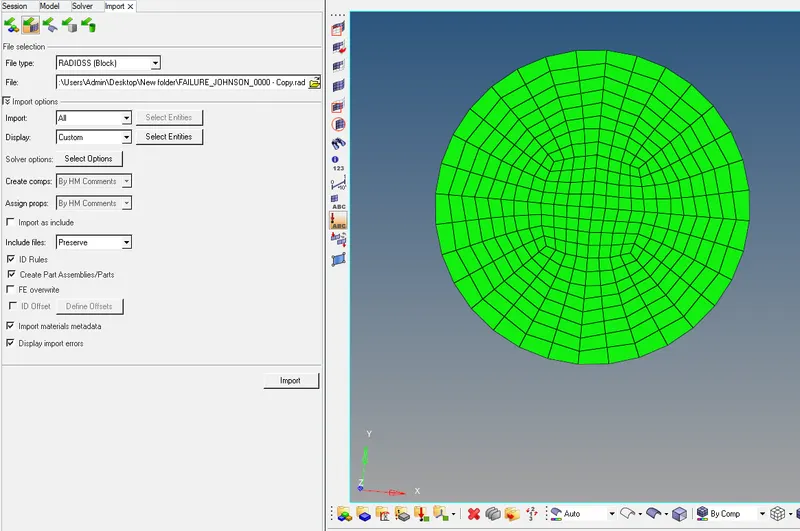
Open Hyper mesh, go to >> import >> solver deck option >> browse File > Import. The “FAILURE_JOHNSON_0000.rad” file is selected and “imported” as shown below.
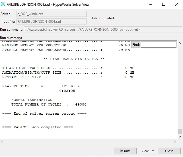
After accessing Hyperview, we should input the simulation file. For this, use h3d file that was generated when RADIOSS processed the starter file.
It is generated in the files swhich are shown in the picture above. After selecting it, we can click 'apply'
After accessing Hyperview, we are asked to input the simulation file. For this, we shall be using the h3d file that was generated when RADIOSS processed the starter file (Law2_epsmax_failure.h3d). It should be generated in the same folder. After selecting it, we can click 'apply'. Doing so generates the simulation animation
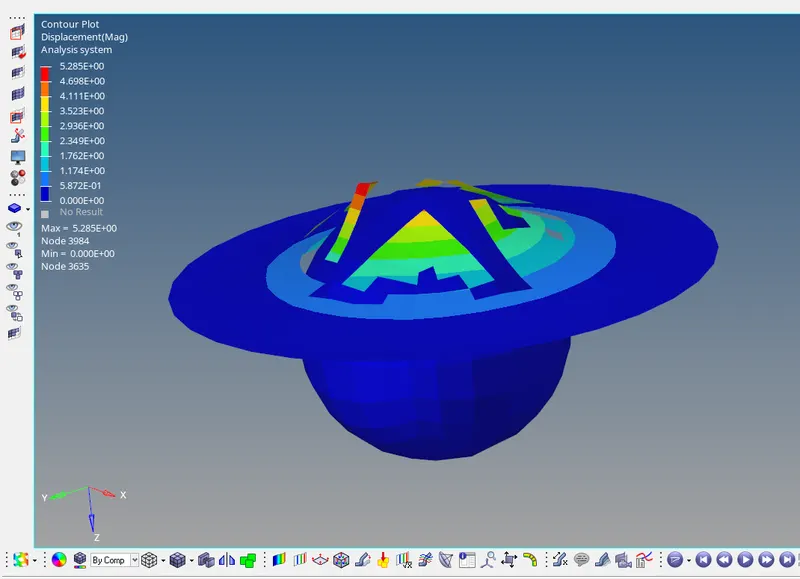
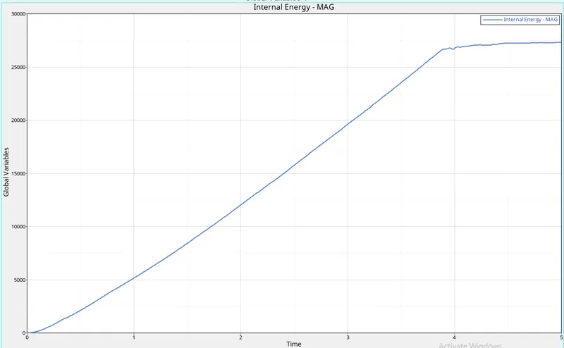
We can change what is being represented by selecting the 'contour' option in the toolbar. In this case, we can change the result type to 'Von Mises' and change the averaging method to simple. Doing so creates the Von Mises stress contours as shown belowe_0000.rad
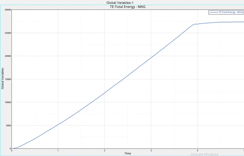
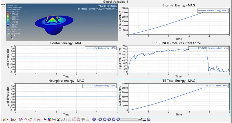
CASE 2
The process is repeated with slight changes. Just as last time, we import “FAILURE_JOHNSON_0000.rad” via the solver deck.
This time, we make some changes to the fail/JOHNSON card. It can be accessed via the model tab, under the “Failures” submenu.
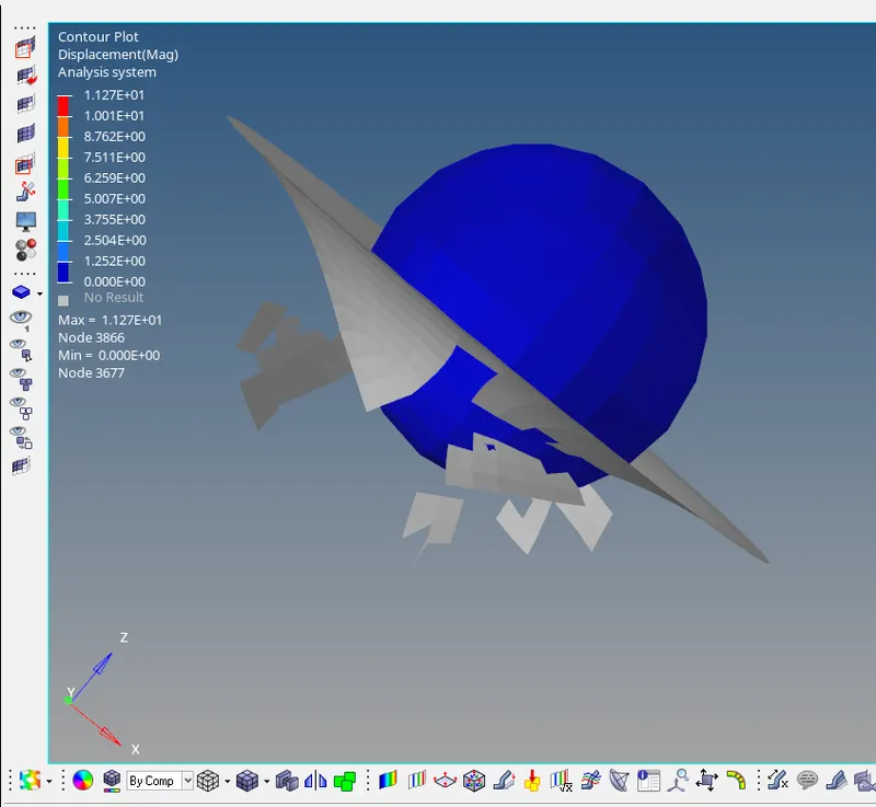
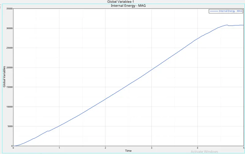
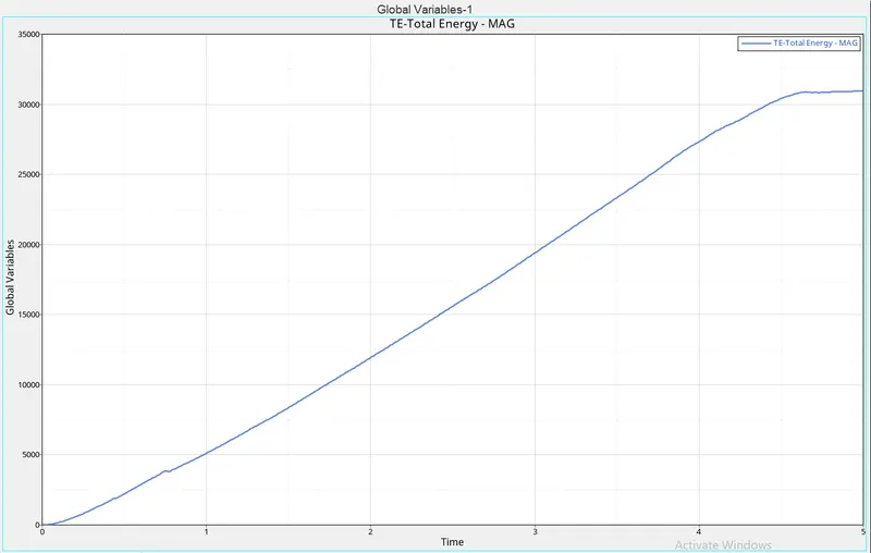
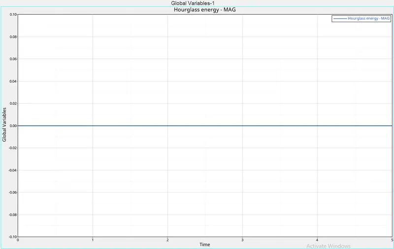
The following values are assigned as shown below (Ifail_sh = 1, Dadv = 1, Ixfem = 1)
Ifail = 1,which determines the Shell element Failure method. So there are two ways in which we can see the element failing, the element will either get deleted or in some cases the cracking occurs according to the material properties.
Ixfem: In this, we can choose that if there is any element that is failing we want that element to delete or we want the element to be crack.We are going to take Ixfem=1. Which allow failed element to cracked not to delete.
Dadv :It gets activated when we have taken Ixfem=1. We are going to takeDadv=1. Which gives the criteria that how much an element can get break into small pieces. If it goes beyond the limit the element gets deleteure
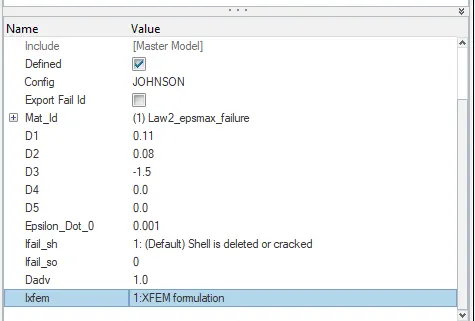
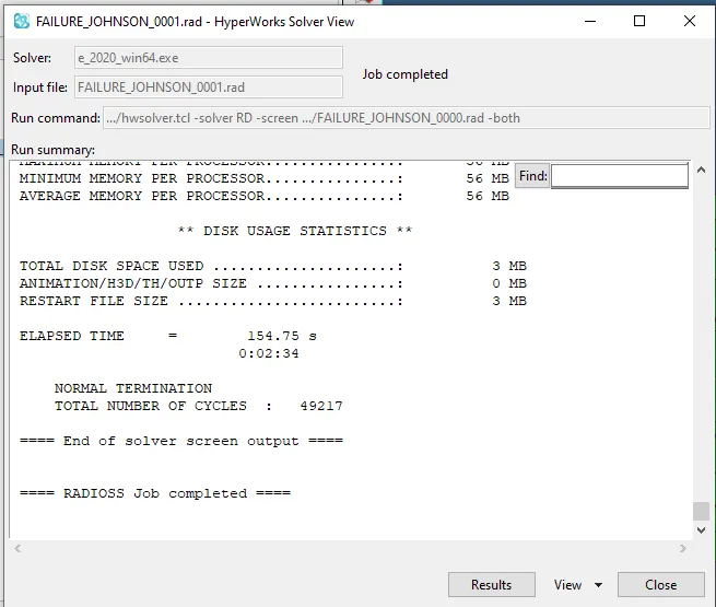
CASE 3
Again, we need to switch to Hyper works and import the solver deck file “Law2_epsmax_crack_0000.rad”, the starter file created in the previous case.
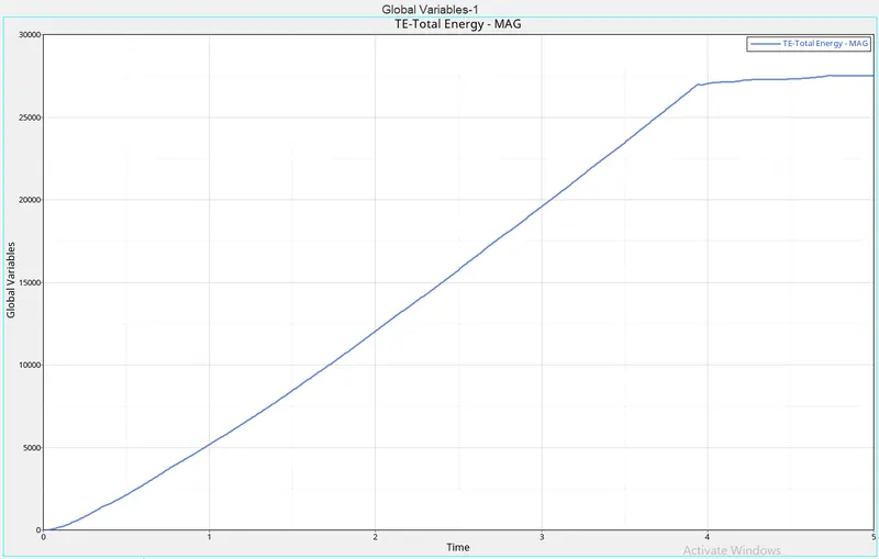
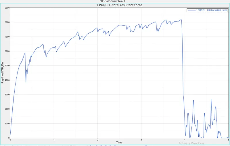
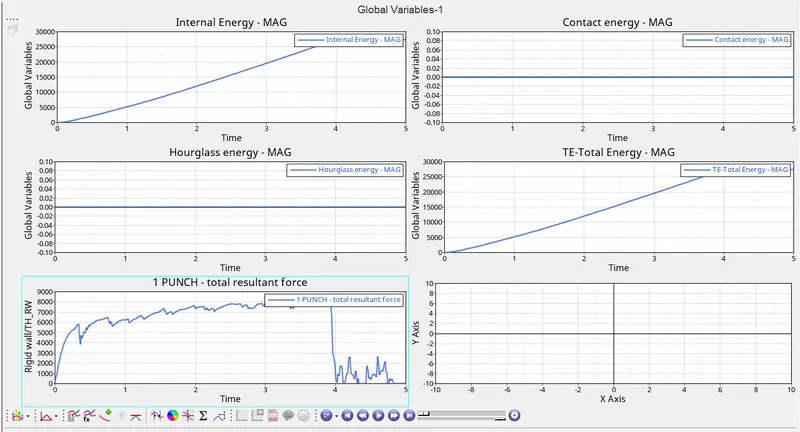
In this case delete the fail/JOHNSON card. Go to Failures > Failure_JOHNSON_1.the limit the element gets deleted
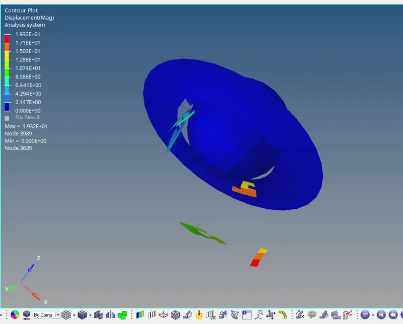
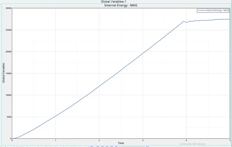
CASE 4
In this case, import the case 3 starter file - Law2_epsmax_nofail_0000.rad.
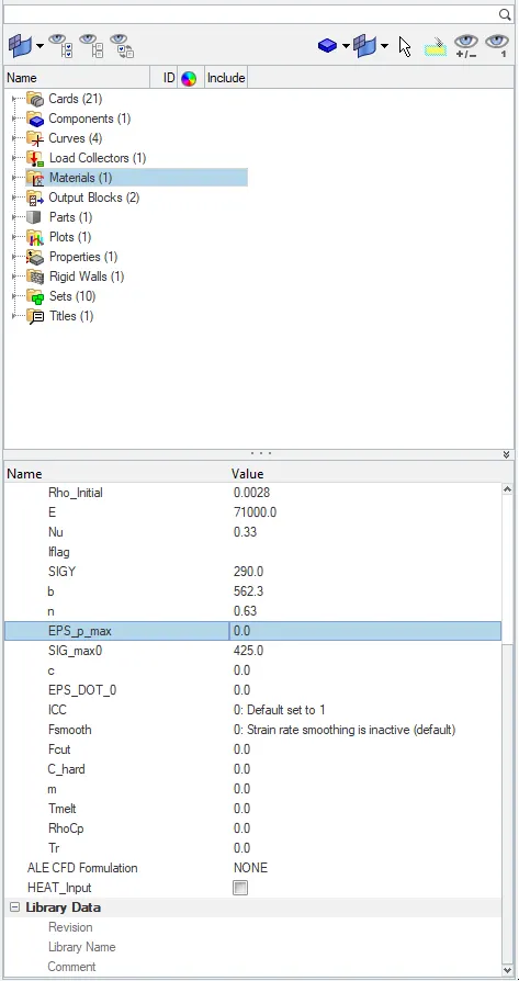
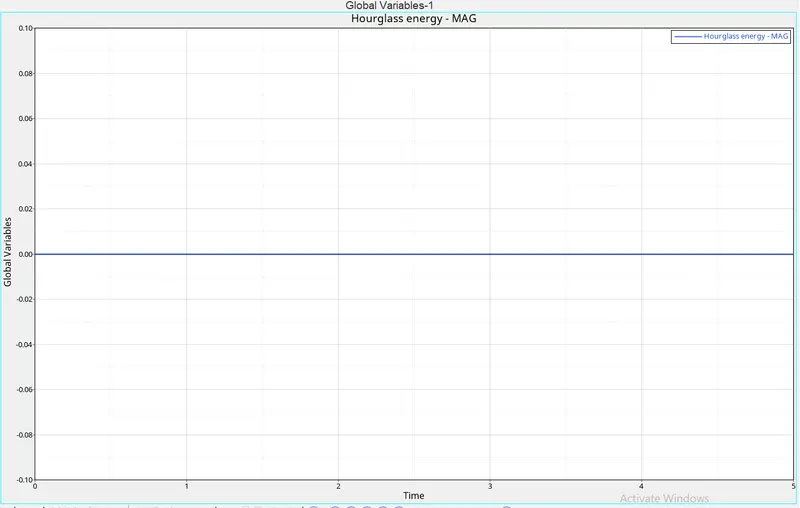
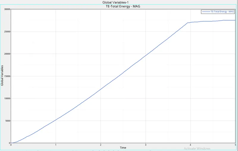
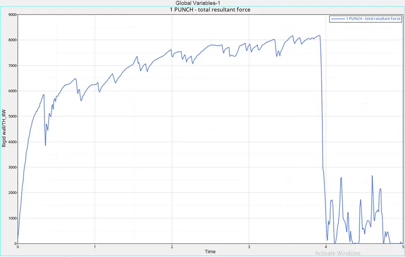
This time, delete the EPS_p_max value (make it as 0). Going to the model tab, we can go to Materials > Aluminium as shown below
CASE 5
In this case import the main starter file - FAILURE_JOHNSON_0000.rad.
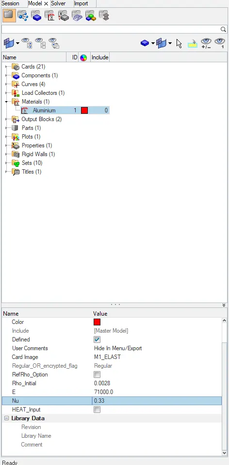
After that, go to Materials card > Aluminium and change the card image to M1_ELAST, which is Law 1.
Also set the values for Rho_Initial, E & Nu as follows:
Rho_initial = 0.0028, E = 71000.00, nu = 0.33.
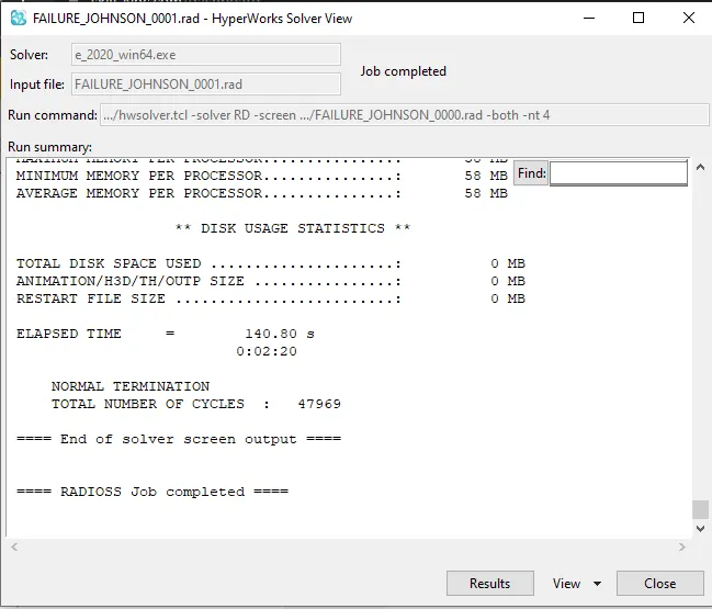
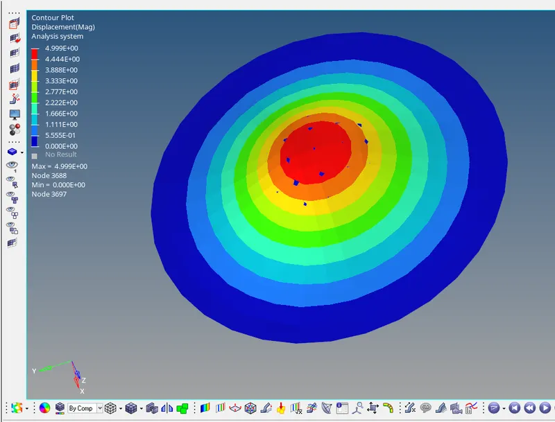
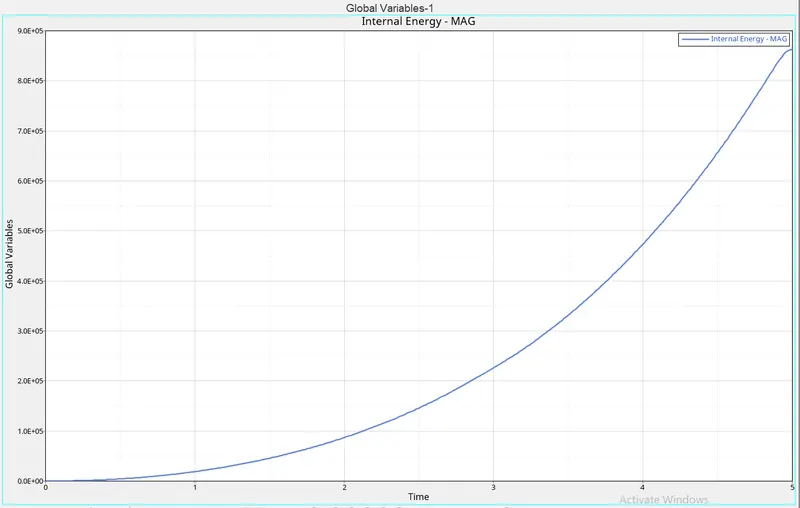
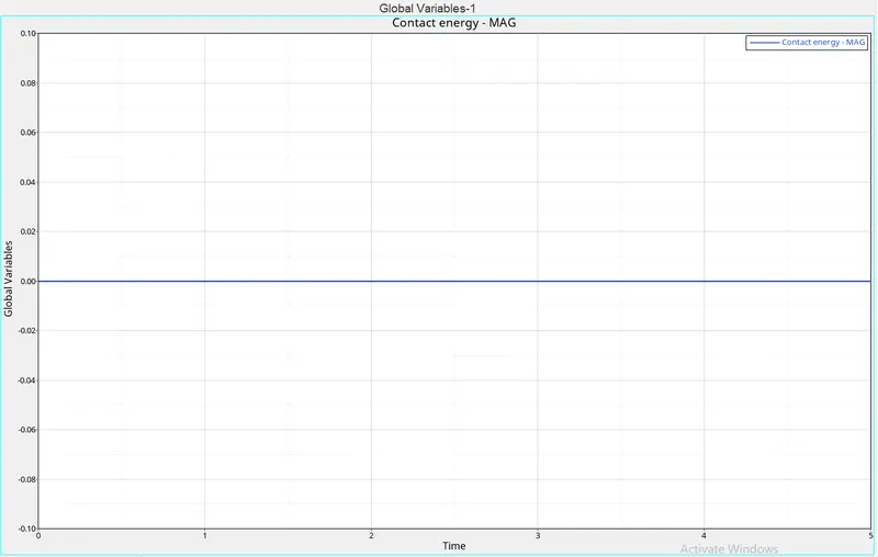
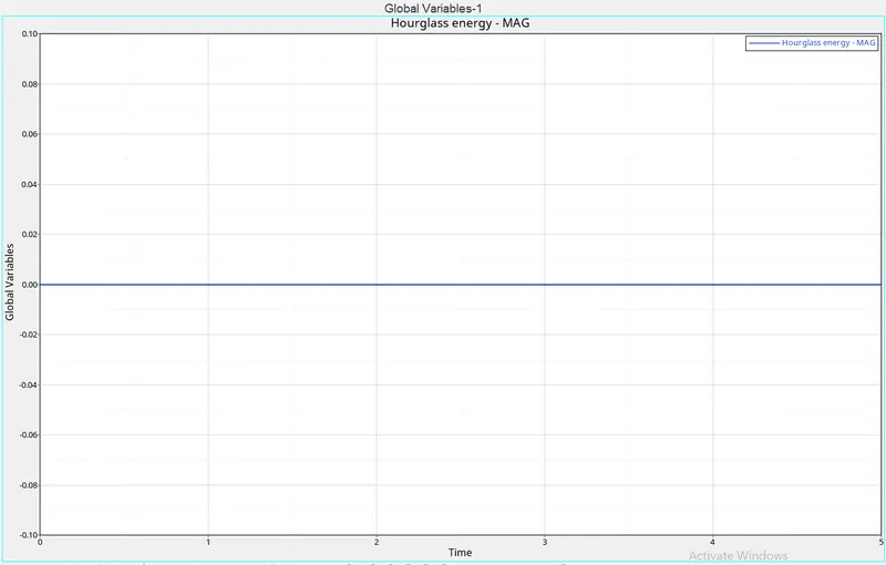
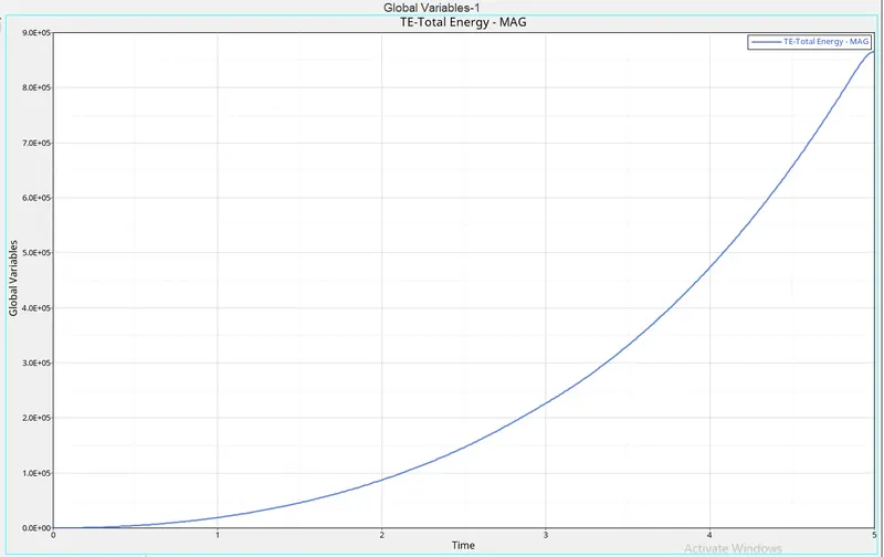
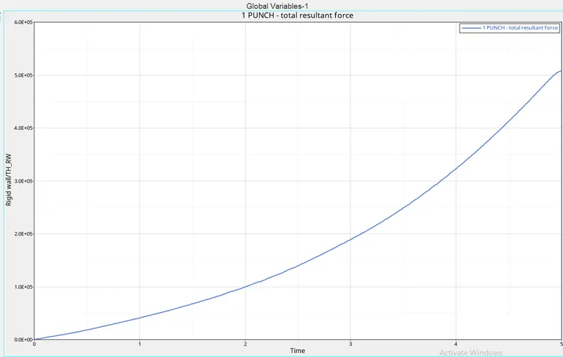
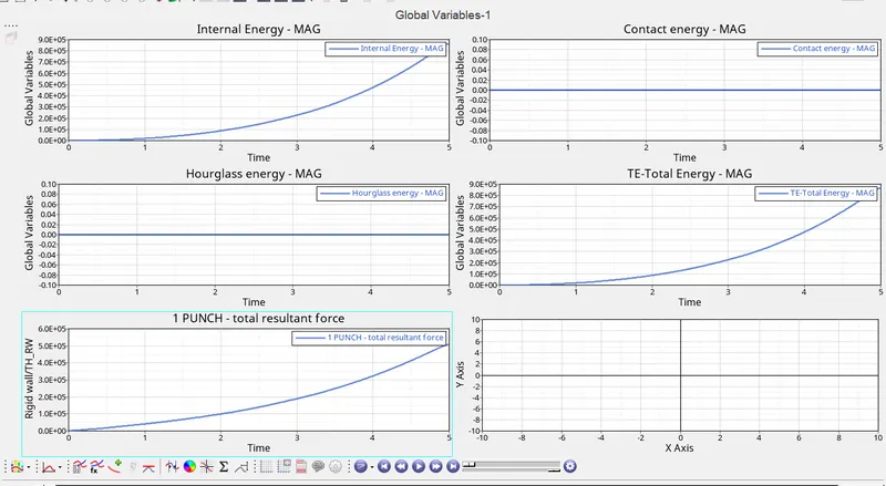
CASE 6
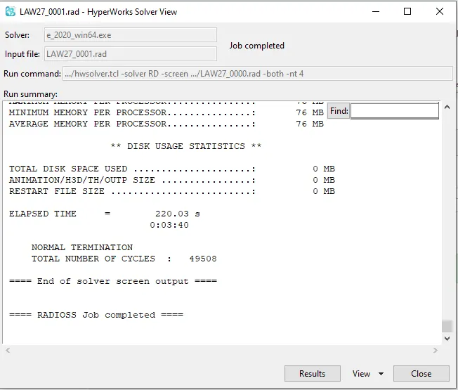
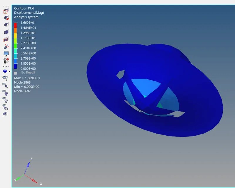
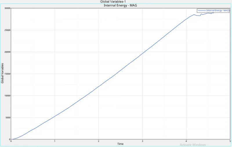
In this case, import the 'LAW27_0000.rad' file.
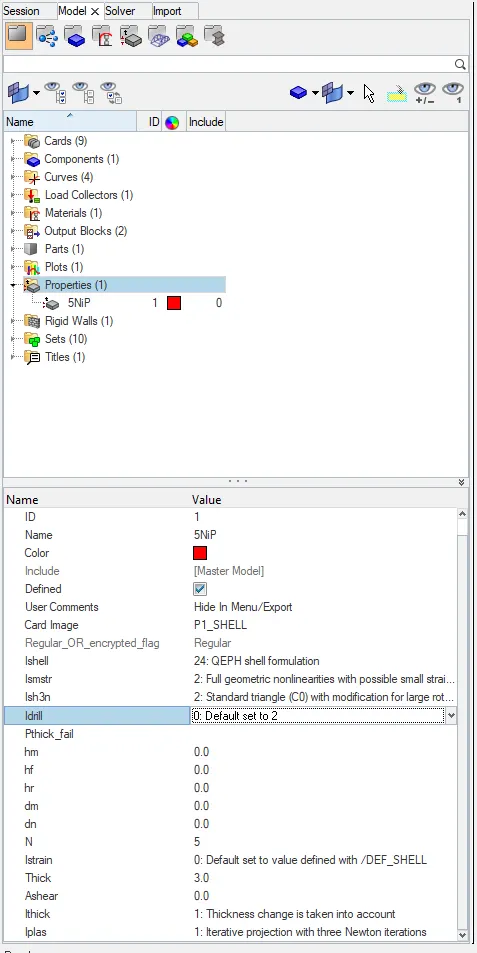
We need to use recommended shell properties in this case. Go to Properties > 5NiP. Now, we can look at the utility window and set the following attributes as follows:
I_shell=24, I_smstr=2, I_sh3n=2, N=5, I_thick=1, I_plas=1
Rho_initial = 0.0028, E = 71000.00, nu = 0.33.
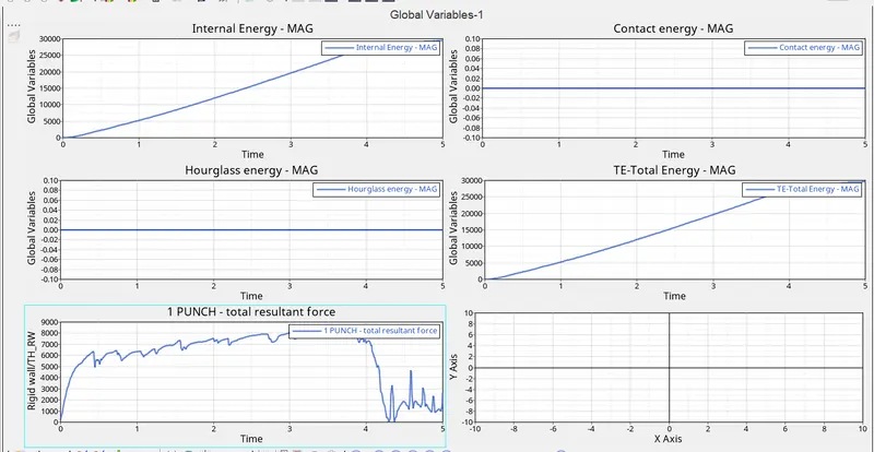
CASE 7
In this case import 'LAW27_0000.rad' again. We shall be editing certain attributes in this case.
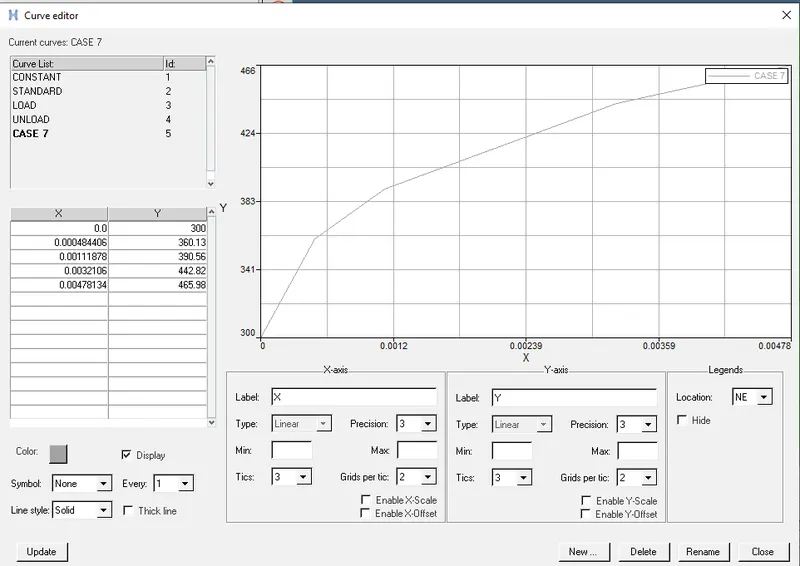
Go to the model tab and here, we shall be creating a new curve (as per instructions given in the week-4, Materials 7 video). Right-Click >> Create >> Curve
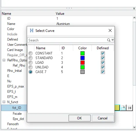
Initially, there are 4 curves, we are adding the new curve named CASE7.
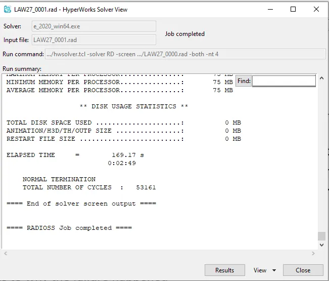
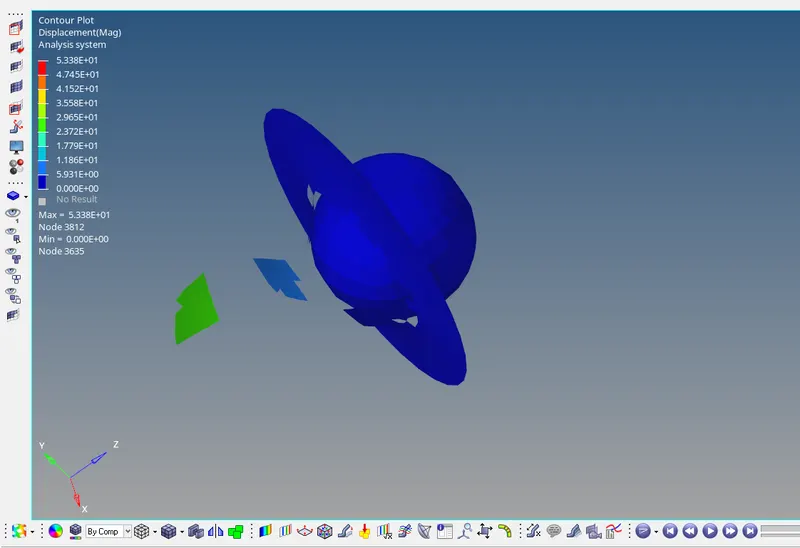
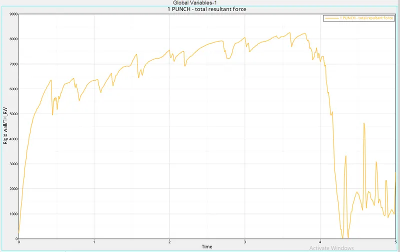
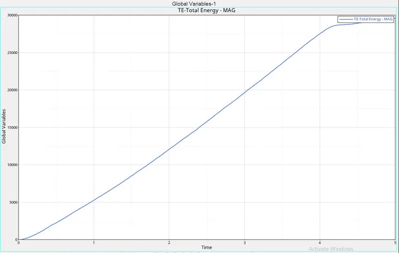
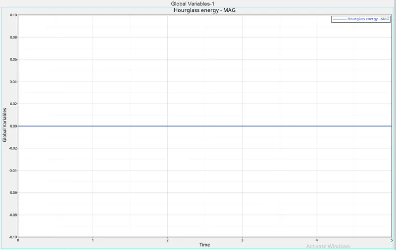
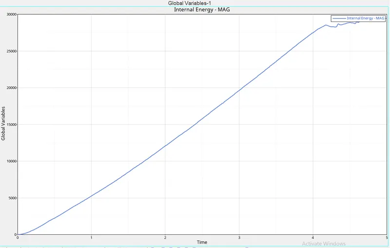
| Case | Material | Simulation name | Energy error (%) | Simulation time (s) | ) Number of cycles | Maximum stress value (MPa) | Element behaviour |
| 1 | Law 2 (Johnson-Cook model) | EPS_max_failure | 0.2 | 73.61 | 49480 | 287.6 | Deleted |
| 2 | Law 2 (Johnson-Cook model) | EPS_max_failure_Crack 4 | 4 | 75.86 | 49379 | 29407 | Cracks first then deleted |
| 3 | Law 2 (Johnson-Cook model) | EPS_max_nofail | 0.8 | 82.56 | 49405 | 270.5 | Deleted |
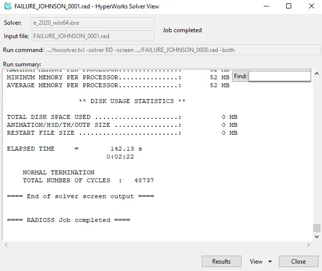
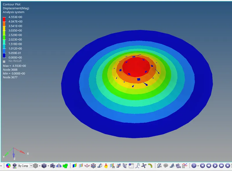
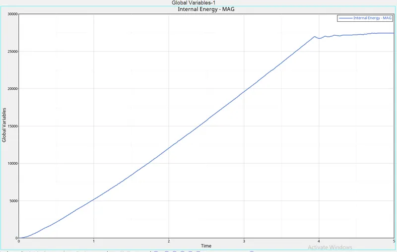
| 4 | Law 2 (Johnson-Cook model) | Law2 | 3 | 73.42 | 48737 | 424.7 | preserved |
| 5 | Law 1 (linear elastic material) | Law1 | 0.3 | 70.33 | 47769 | 10860 | preserved |
| 6 | Law 27 ( brittle failure model) | Law 27 | 1 | 78.31 | 49364 | 277.3 | Deleted |
| 7 | Law 36 (elasto-plastic materia) | Law 36 | 0.8 | 76.07 | 52237 | 1286 | Deleted |