Challenge

Assignment 4-RADIOSS Material Laws Challenge

SShaik Basheeruddin Khasim24 Sept 2021

AIM:To run the simulation of the given model and compare the model with the different materials Laws.

Objective:The objective of this project is as follows.

To run the model as it is and name it Law2_epsmax_failure.
In/FAIL/JHONSON,change Ifail_sh=1,Dadv=1,and Ixfem=1 values and run the model as Law 2_epsmax_crack.
Delete the /FAIL/JHONSON card and run the model as Law2_eps,ax_nofail.
Delete the values of EPS_p_max and run the model with name Law2
Convert this material model to Law1 elastic with the same density ,E,Nu,and run the simulation.
Convert this material into Law36 with the values given and run the model.
Open the LAW27_0000.rad file and change the shell properties to recommended shell properties and notice the material card and Johnson cook parameter but different values for EPS based and run the model with Law2.

Case 1:

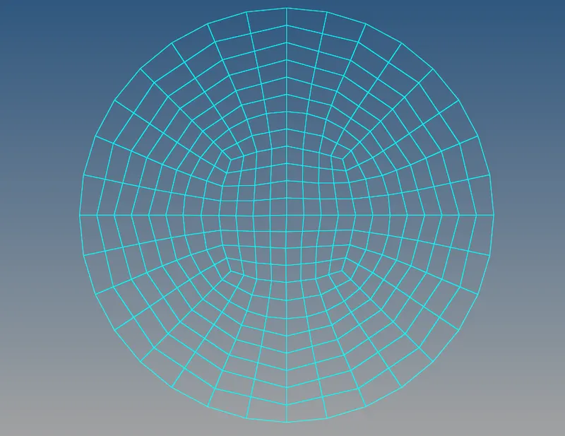
Importing the given model by going to the file>import>slover deck>Jhonson 0000.rad statter file and import into the GUI.
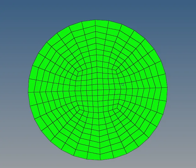
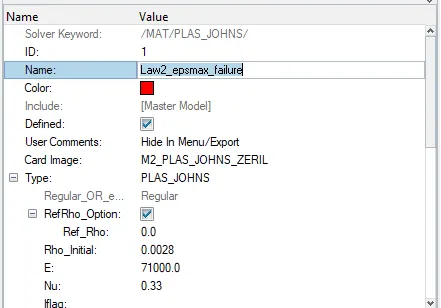
After importing change the model into Wire frame geomentry and Open material card in the Tab area, Model Browser >> See the Values and change the Name from Aluminum to Law2_epsmax_failure.
Now Go to the Analysis Panel >> Select Radioss >> Select the input file and save the file in a new folder naming Case 1 >> Check include connectors box >> In Options, enter “-nt 4”. >> Click on Radioss.
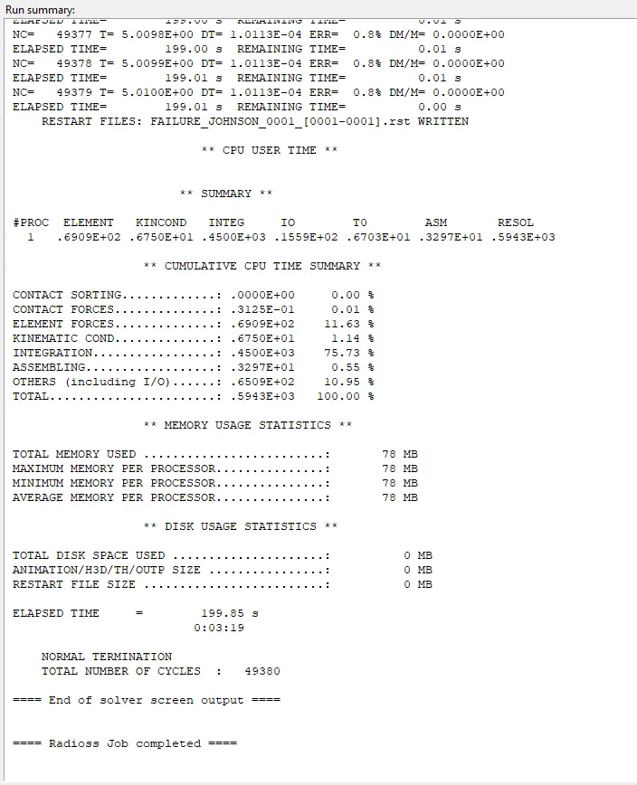
A new window will be opened simulating the model and the result will be displayed in the same window (i.e if the simulation is successful or not)aw2_epsmax_failure.
A new window will be opened simulating the model and the result will be displayed in the same window (i.e if the simulation is successful or not)

For Case 2:

In the Model Broswer, Check for the Failure card >> Click on Failure_JOHNSON_1 >> Change the Values of Ifail_sh =1 , Dadv =1 and Ixfem =1.
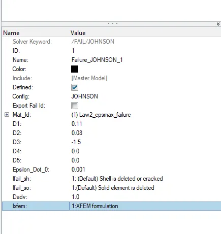
The Failure card is set.Go to the Material Cards >> Select the Material >> Change the name to Law2_epsmax_crack.
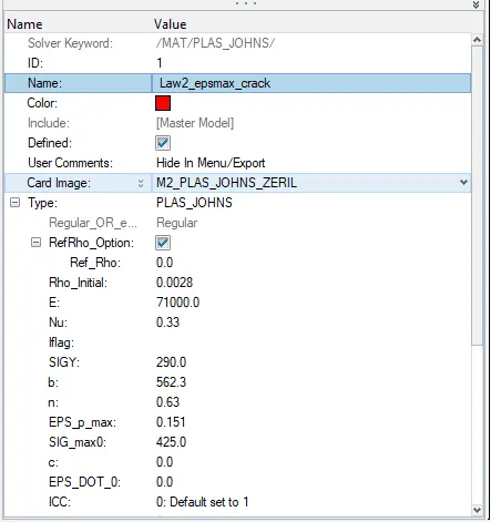
Now, go to the Analysis panel, click Radioss >> Select the input file and save the file in a new folder naming Case 2 >> Check include connectors box >> In Options, enter “-nt 4”. >> Click on Radioss.
The Simulation is run successfully.Go to the Material Cards >> Select the Material >> Change the name to Law2_epsmax_crack.
Now, go to the Analysis panel, click Radioss >> Select the input file and save the file in a new folder naming Case 2 >> Check include connectors box >> In Options, enter “-nt 4”. >> Click on Radioss.
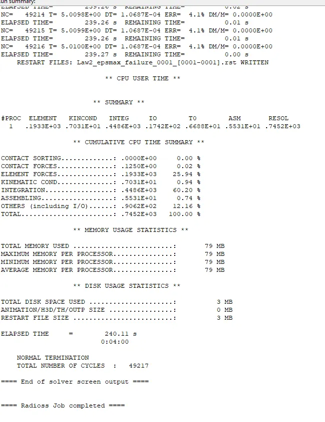
The Simulation is run successfully.

For Case 3:

To delete the Failure card, Go to the card that you want to delete >> Right-click on it >> Click Delete.
The Card will be deleted.
Go to the Material Card, Click the Material >> Change the name to Law2_epsmax_nofail.
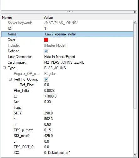
Now, go to the Analysis panel, click Radioss >> Select the input file and save the file in a new folder naming Case 3 >> Check include connectors box >> In Options, enter “-nt 4”. >> Click on Radioss.
The Simulation is executed without any failure.

For case 4: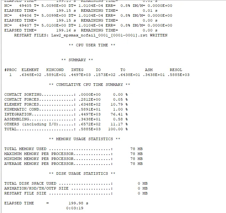

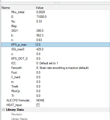
In the Material Card, Check for the EPS_p_max value >> change it to 0.
Now, go to the Analysis panel, click Radioss >> Select the input file and save the file in a new folder naming Case 3 >> Check include connectors box >> In Options, enter “-nt 4”. >> Click on Radioss.
The Simulation is executed without any failure.

For case 5: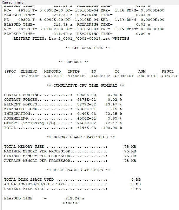

To change the card image to law1, go to the Material card >> click on the material >> Hover on the Card Image >> Select the Dropdown option and Select M1 Elastic >> Give the Rho_ Initial (Density) value as 0.0028, E (Young’s Modulus) value as 71000, Nu (Poisson’s Ratio) value as 0.33.
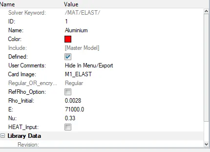
Now, go to the Analysis panel, click Radioss >> Select the input file and save the file in a new folder naming Case 3 >> Check include connectors box >> In Options, enter “-nt 4”. >> Click on Radioss.
The Simulation is executed without any failure.

For case :6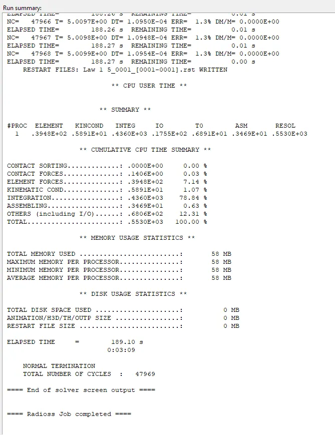

In this case, import the 'LAW27_0000.rad' file.
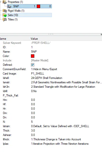
We need to use recommended shell properties in this case. Go to Properties > 5NiP. Now, we can look at the utility window and set the following attributes as follows:

I_shell=24, I_smstr=2, I_sh3n=2, N=5, I_thick=1, I_plas=1
The material criteria are given. Now, go to the Analysis panel, click Radioss >> Select the input file and save the file in a new folder naming Case 6 >> Check include connectors box >> In Options, enter “-nt 4”. >> Click on Radioss.

Case 7:

Open the New File as Previously mentioned method. The FileName is “LAW27_0000.rad”.
Check the material properties and change the values if there’s any change. Change the Name to Law 27.
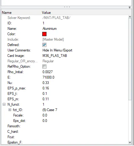
Similar to case 5, change the Material Card to Law 36 Plastic Tab >> Change the Name to Law36 >> Give the Values of Rho_Initial (Density ) value as 0.0027, E (Young’s Modulus ) value as 71000, Nu (Poisson’s Ratio) value as 0.33, EPS_p_max (Failure Plastic Strain) value as 0.16, EPS_t (Tensile Plastic Strain) value as 0.1, EPS_m (Tensile Plastic Strain) value as 0.11, N_Funct (number of Functions) as 1 >> To specify fct_ID a Curve must be plotted.
To Plot the Curve, Go to the Curves tab in the Model Browser >> Right Click on the Curves >> Click Create >> Click New >> Give a Name to the Curve to be Plotted >> Click Proceed >> Give X and Y Coordinates >> Click Update.
Now go to the material card again and click on the curve option in the fct_ID >> Select the New Curve Created >> Click Ok.
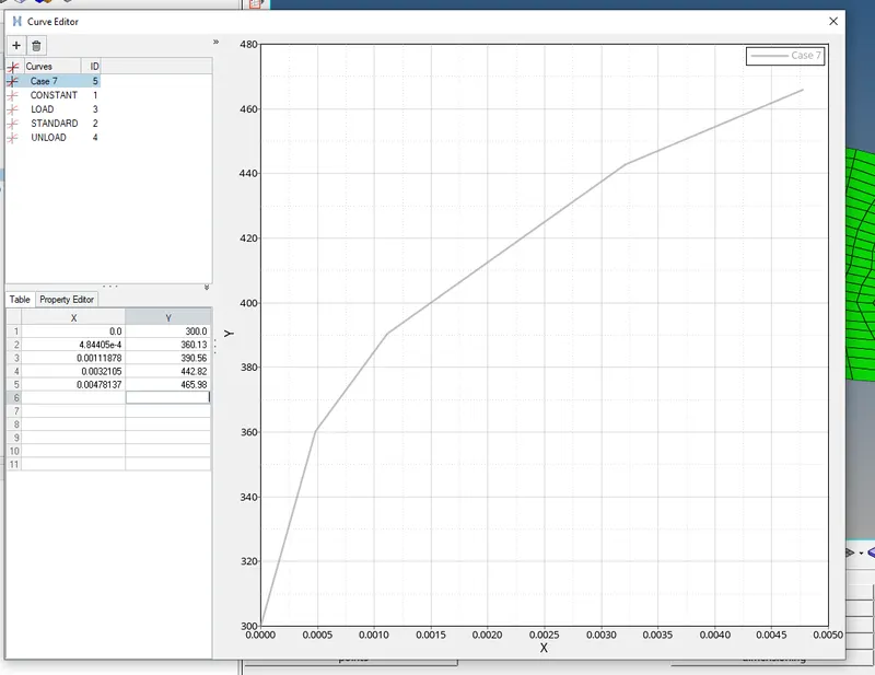
The material criteria are given. Now, go to the Analysis panel, click Radioss >> Select the input file and save the file in a new folder naming Case 7 >> Check include connectors box >> In Options, enter “-nt 4”. >> Click on Radioss.

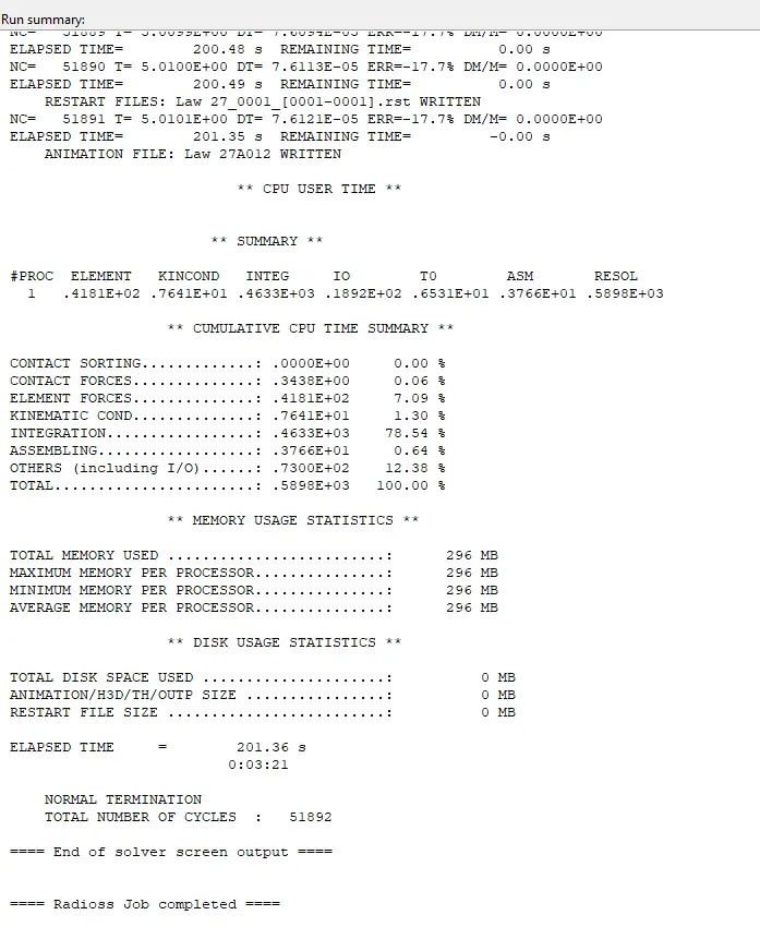
Comparing the Results of the cases1 to case 7 in Hyperview and Hypergraph 2D:

Case 1:

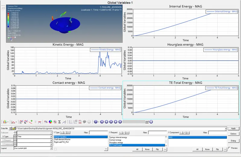
There is a linear increase in both Total energy and Internal energy but there is a small deflection in the internal energy which is a minute deflection.
Hourglass Energy, Kinetic Energy, and Contact Energy is constant throughout the process.
There is a small rise in kinetic energy at the period when the Internal Energy got deflected.

Case 2:

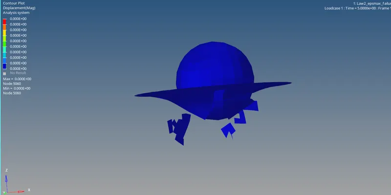
There is a linear increase in both Total energy and Internal energy but there is a small deflection in the internal energy which is minute deflection and the deflection is delayed compared to case 1.
This delay in deflection is due to the element deletion due to failure by cracking.
Hourglass Energy, Kinetic Energy, and Contact Energy is constant throughout the process.
There is a small rise in kinetic energy at the period when the Internal Energy got deflected.

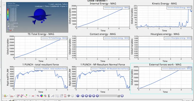
Case 3:

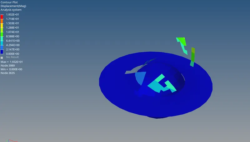
There is a linear increase in both Total energy and Internal energy but there is a small deflection in the internal energy which is a minute deflection.
Hourglass Energy, Kinetic Energy, and Contact Energy is constant throughout the process.
There is a small rise in kinetic energy at the period when the Internal Energy got deflected.

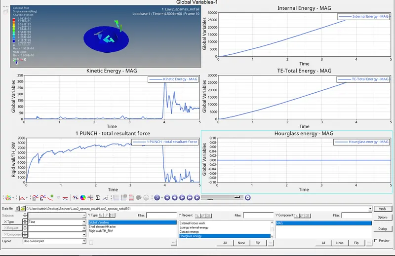
Case 4:

There is an exponential increase in both Total energy and Internal energy.
Hourglass Energy, Kinetic Energy, and Contact Energy is constant throughout the process.

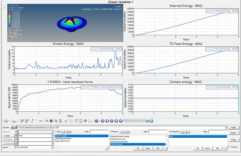
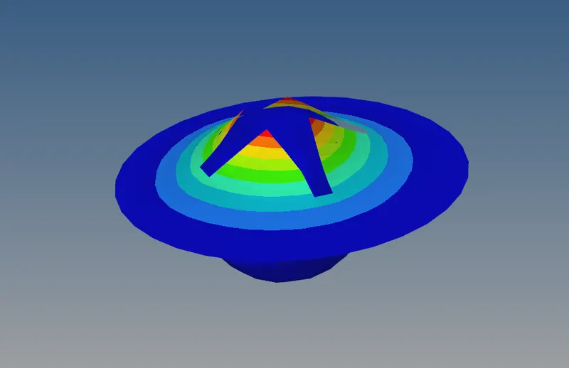
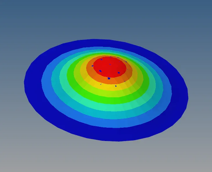
Case 5:

There is a linear increase in both Total energy and Internal energy but there is a small deflection in the internal energy which is a minute deflection.
Hourglass Energy, Kinetic Energy, and Contact Energy is constant throughout the process.
There is a small rise in kinetic energy at the period when the Internal Energy got deflected.

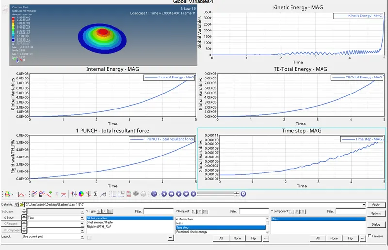
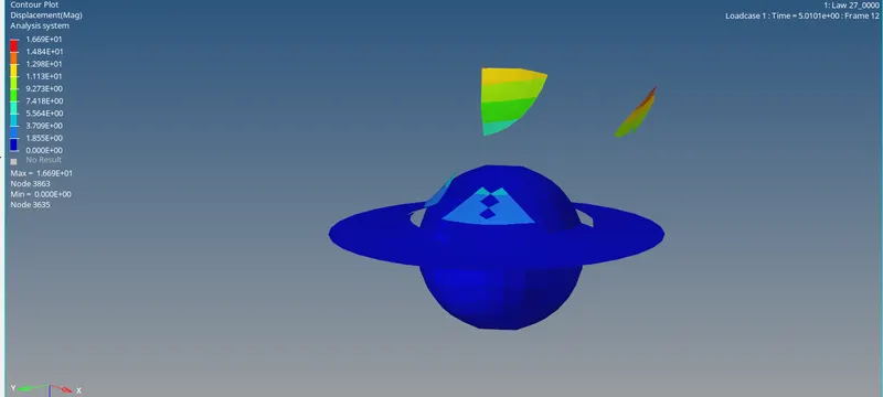
Case 6:

There is a linear increase in both Total energy and Internal energy but there is a deflection in the internal energy.
Hourglass Energy, Kinetic Energy, and Contact Energy are constant throughout the process.
There is a small rise in kinetic energy at the period when the Internal Energy got deflected.

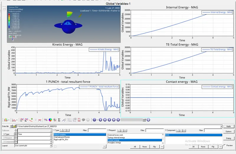
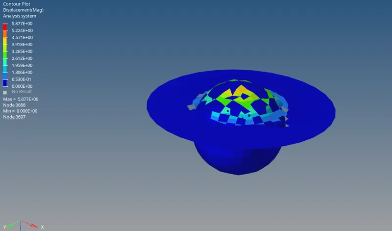
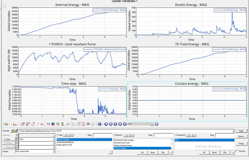
Case 7:

There is a linear increase in both Total energy and Internal energy.
Hourglass Energy, Kinetic Energy, and Contact Energy is constant throughout the process.

CASE	No of cycles	Mass Energy	Final Energy	Solver Simulation(sec)
Case 1	49379	0	0.8%	199.0
Case 2	49216	0	4.1%	239.25
Case 3	49407	0	0.8	199.16
Case 4	49303	0	1.1%	211.40
Case 5	47968	0	1.1%	188.27
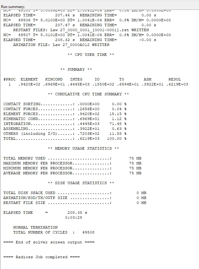
Case 6	49507	0	0.8%	208.37
Case 7	51891	0	-1.8%	201.35

Results:

The simulation is completed and cases are compared with each other.

Terms Used:

Law1:

Law 1 defines an isotropic, linear elastic material using Hooke's Law. This law represents a linear relationship between stress and strain. It is not be used for parts undergoing large deformation.

Law2:

This law represents an isotropic elastoplastic material using the Johnson-Cook material model. This model expresses material stress as a function of strain, strain rate &Temperature.

Law27:

This Law combines an isotropic elastoplastic Johnson-Cook material model with an orthotropic brittle failure model. Material damage is accounted for before failure. Failure and damage occur only in tension. This Law is applicable only for shells. It deals with a Brittle failure.

Law36:

This Law models an isotropic elastoplastic material using user-defined functions for the work hardening portion of the stress-strain curve. Material Plasticity curves can be given for up an arbitrary number of strain rates.

Ixfem:

Ixfem is a deciding factor in cracking the element.

There’s a possibility to separate the crack initiation and advancement criteria entended to other compatible failure models.

Total Energy:

The total energy of a system is the sum of kinetic and potential energy.

Contact Energy:

The frictional energy is already included in the slave energy and the master energy and hence also in the sum of slave/master energy. Thus, one gets the energy needed to prevent penetration between the contact partners by subtracting the frictional energy from the sum of slave/master energy. In the absence of friction, the slave energy and the master energy should be close in magnitude but opposite in sign and the sum of slave/master energy should equal the stored energy.

Internal Energy:

The internal energy of a thermodynamic system is the energy contained within it. It is the energy necessary to create or prepare the system in any given internal state. It does not include the kinetic energy of motion of the system as a whole, nor the potential energy of the system as a whole due to external force fields, including the energy of displacement of the surroundings of the system. It keeps account of the gains and losses of energy of the system that are due to changes in its internal state. The internal energy is measured as a difference from a reference zero defined by a standard state. The difference is determined by thermodynamic processes that carry the system between the reference state and the current state of interest.

Kinetic Energy:

In physics, the kinetic energy (KE) of an object is the energy that it possesses due to its motion. It is defined as the work needed to accelerate a body of a given mass from rest to its stated velocity. Having gained this energy during its acceleration, the body maintains this kinetic energy unless its speed changes. The same amount of work is done by the body when decelerating from its current speed to a state of rest.

Conclusions:

Many things are learned during this project.

Learned how to simulate the model.
Learned how to check the animation.
Learned how to plot the graph using HyperGraph.
Learned how to compare the Animations and Graphs.

Assignment 4-RADIOSS Material Laws Challenge

Ship work like this
in your own course.

Talk to a career counsellor

Ship work like thisin your own course.

Talk to a career counsellor

Ship work like this
in your own course.