Assignment 4-RADIOSS Material Laws Challenge
1. Objective:
- To apply the various cases as mentioned in the above question on the given failure johnson cook material.
- To plot the graphs(Post-processing) with respect to the obatined values from those cases.
- To compare the obtained results, from those cases.
2. Software used: Altair Hyperworks Desktop 2020.
3. User profile: Radioss
4. Procedure:
Case 1 (Running the simulation without any change):-
Initially, after opening the hyperworks software the user profile should be selected. For this challenge since analysis should be performed, Radioss
is choosed as an user profile. After choosing the user profile, The solver deck should be imported. The file should be selected & cilck on import.
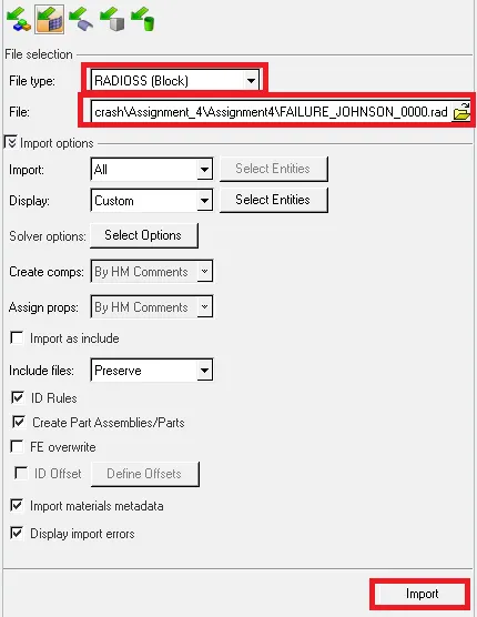
After importing the solver deck, the model appears in the graphical display.
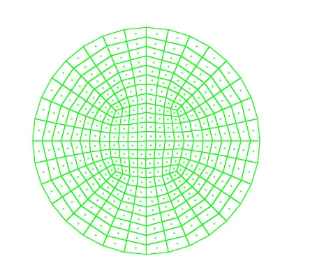
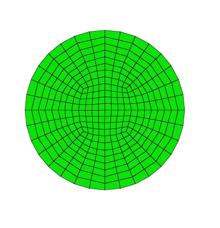
As it is seen in wireframe mode for better visualization, enable the option named "Shaded elements with mesh lines". After enabling it, the given
model appears.
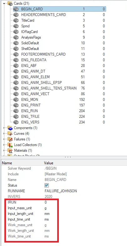
Then in the solver browser some cards are verified, inorder to have clarity on some aspects. Among them, the first card to be checked is "Begin
card". Inorder to check for the unit system. The unit system plays a prominent role for assigning all of the values.
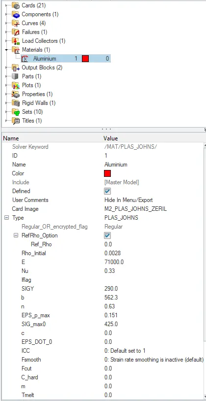
The material card is the next card to be verified, inorder to see the properties assigned to the material. The material card appears as shown in
below fig.
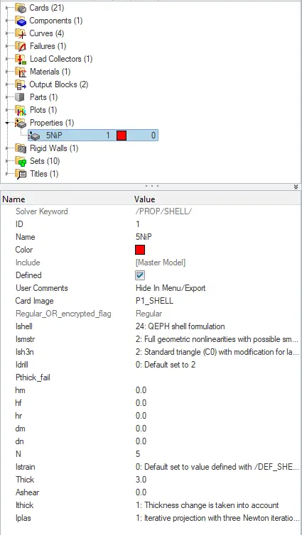
Next card to be verified is property card. In property card, the properties assigned to the given material is seen. The property card with the
assigned parameters appears as shown in fig below.
As mentioned, this case is to be runned as usually with the base values. i.e., running the model without changing any value. The model can be
runned with the help of command named "radioss" in the analysis panel. After opening the radioss panel, the file should be assigned with in some
location. Then by clicking "save as", the files will be saved in that locations.
To increase the speed of the simulation, in the options bar which is highlighted in the fig below, a value entered as "-nt 4", in which nt depicts the
number of threads. And 4 depicts the number cores in the system takes the task simultaneously. Then click on "Radioss" to run the model.

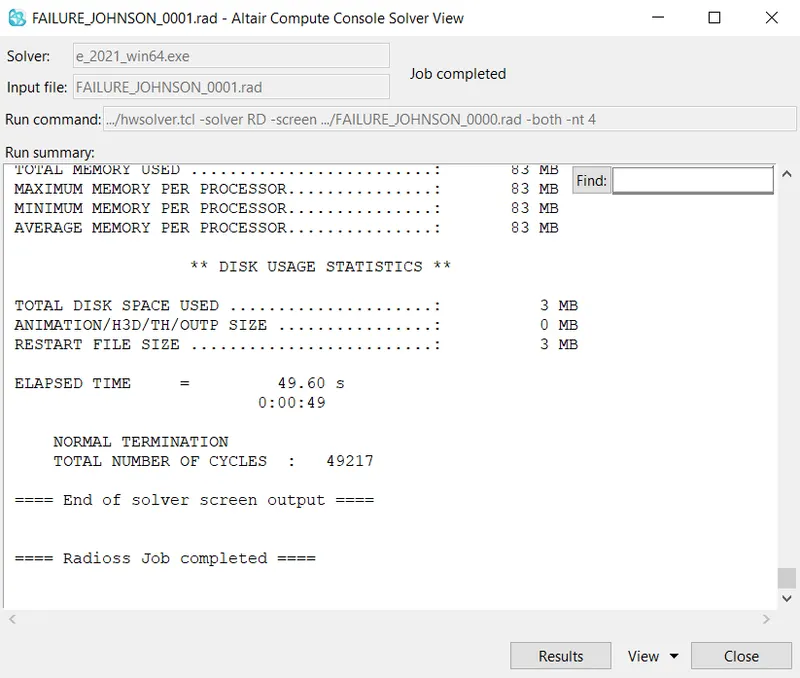
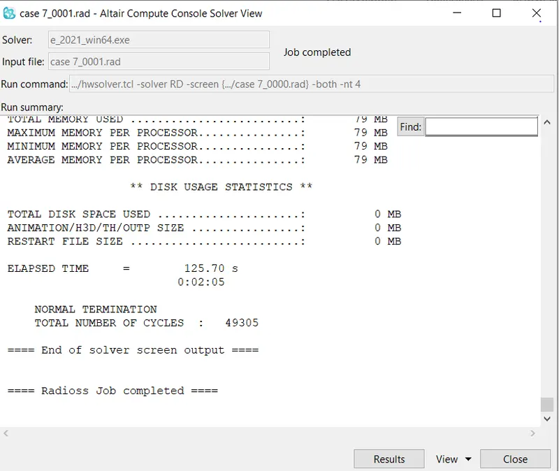
It takes few moments to run the simulation and generate the animation files, time history files. After completing the job of the radioss, a pop-up
appears as shown in fig.
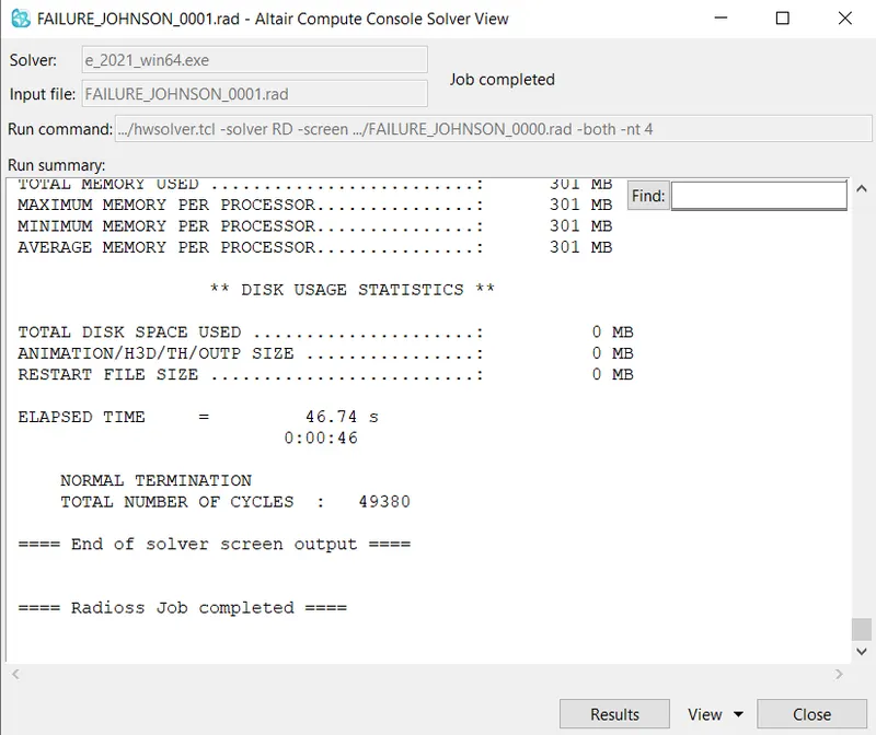
As the running is completed, the location which is assigned before running. In that location, the files are stored.
Among those files, the 0001.out file is opened in the notepad++, which indicates the results in the form of numerical values(such as energy error,
mass error, kinetic energy, internal energy, etc) as shown in fig.
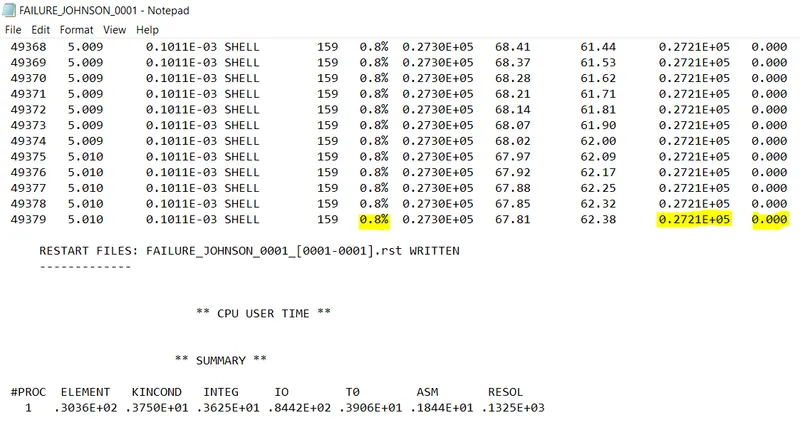
The obtained last cycle values are:
energy error = 0.8%
Internal energy = 0.2730E+05 KJ
Kinetic energy = 67.81 KJ
External work = 0.2721E+05 KJ
Mass error = 0
elapsed time = 46.74 s
Total number of cycles = 49380
Then the 0001.rad file is opened in the note pad, which shows the Tfrequency, run time(Tstop) values as shown in fig.
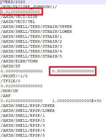
The next step is to view the simulation. This is done by switching on to other window. In this window, the h3d file is imported and applied in the
hyperview. The hyperview panel appears as shown in fig.
Note:
- Always when we switched on to new window, the hyperview panel is enabled by default. To plot the graphs(i.e., post processing), the hypergraph 2D panel should be enabled by the user.
- The h3d file is a combination of all animation files.

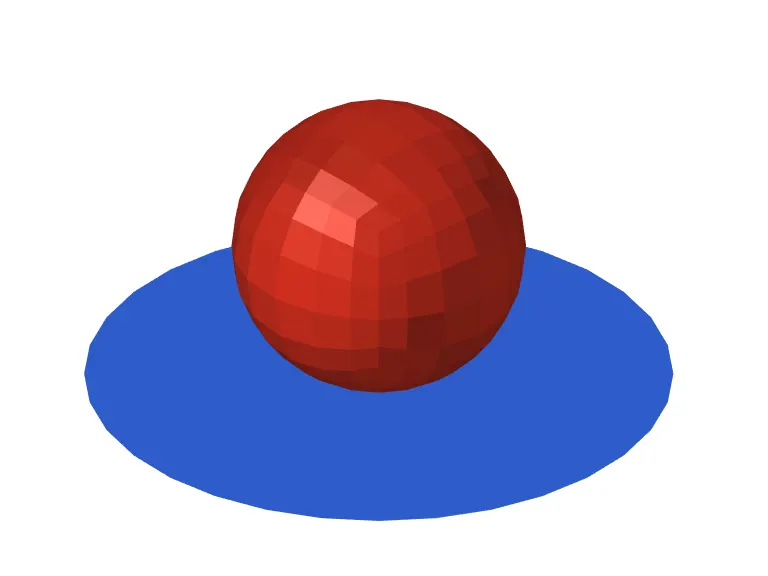
After importing the h3d file in the hyperview panel, the model in the graphical display appears as shown in fig.
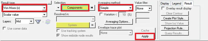
To run the simulation, the contour panel should be enabled. Which appears as shown in fig above. In this panel, the parameters such as result type
as von misses, selection of components, selection of averaging method, and clicking on apply.
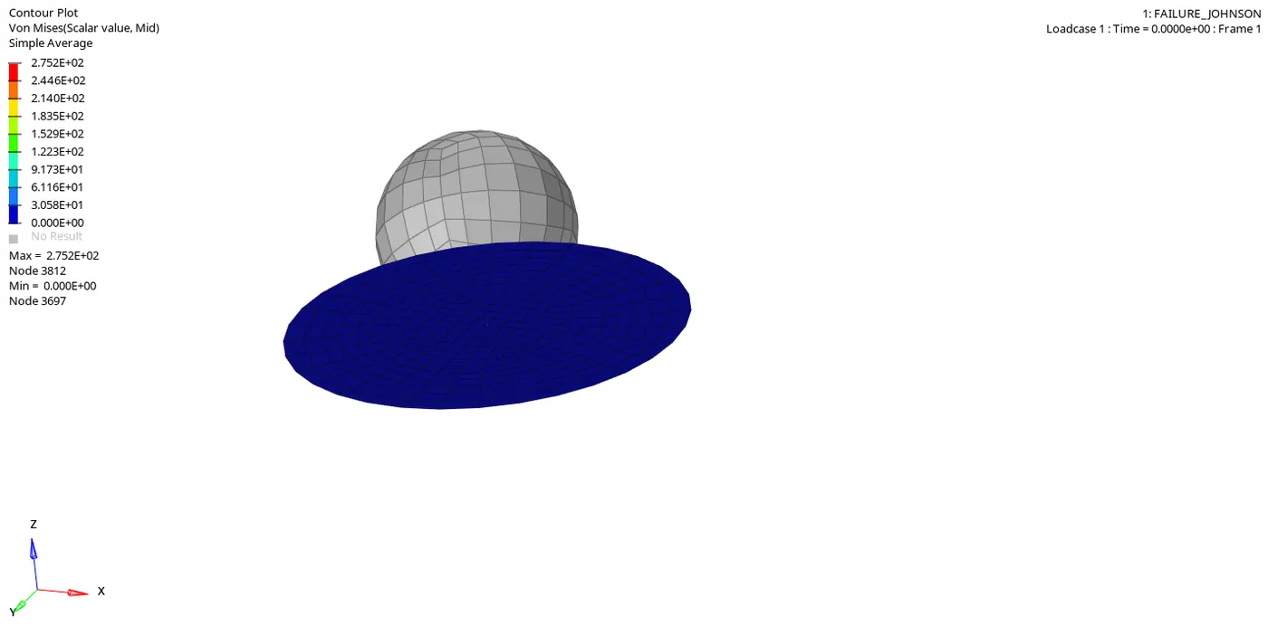
After applying, the model is ready for simulation. The obtained simulation appears as shown in the below animation. Which results in deleting the
elements, because the circular plate is assigned with the law 2. As it is assigned with material law 2, the plate possess both elastic & plastic
behavior. The maximum von-mises stress is seen in the below animation.
Post-processing:
The next step is to do the post-processing, by plotting the obtained results in the form of various graphs. The first graph to be plotted is rigid wall
forces. This is done by switcing in to the new window & enabling the Hypergraph 2D panel. In this panel, T01(Time history) file is impoted. And the
parameters required for obtaining the result with respect to the rigid wall are selected as shown in fig.

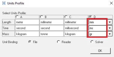
After selecting to apply, a pop-up appears as shown in fig below. Which depicts to mention the unit system. As per the unit system seen in begin
card from solver browser, the units selected are length(milli meter), Time(milli seconds), Mass(grams).
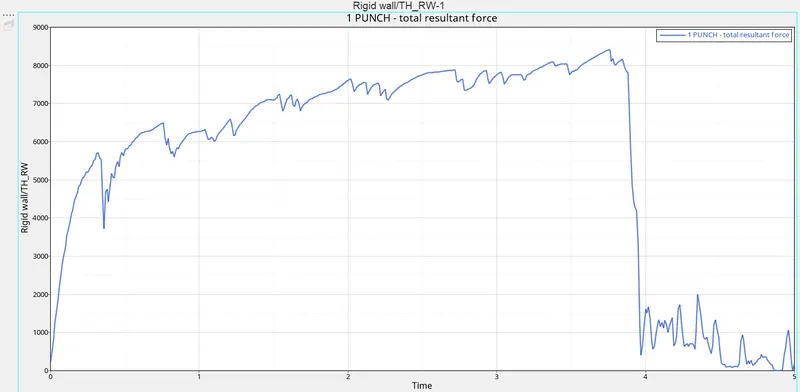
Soon after applying the unit system, the graph is plotted which indicates the rigid wall total resultant force as shown in fig. Initially, the
elemnts start observing the energy, when the spherical shaped rigid sphere hits the given component(Plate shaped). And due to this energy
absobtion, the forces will reach till a peak value as shown in fig 5.17. And after reaching the peak value, the elements will start deleting, Which is
shown in the fall of the rigid wall forces.
The next step is to plot the graph for the energies such internal energy, kinetic energy, Total energy, hourglass energy. So for that, the parameters
are selected in the hypergraph 2D panel as shown in fig. This should be done in the new window.

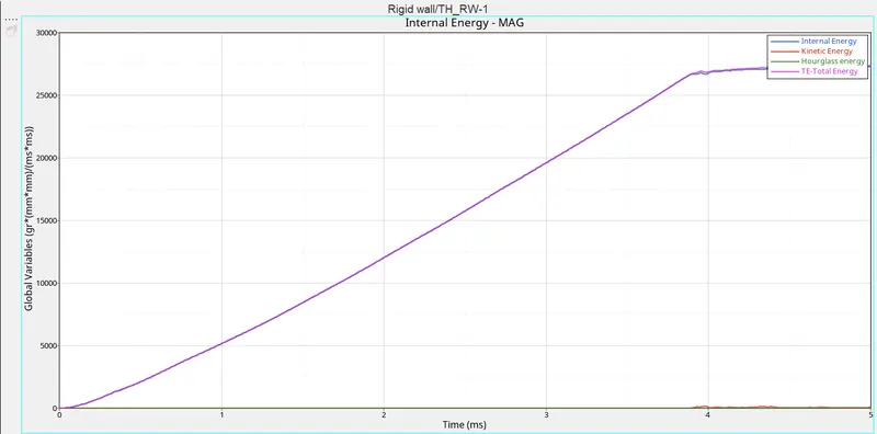
The obtained graph with respect to the requested energies appears as shown in fig. As in this case the johson cook material with the law 2 is
applied and represented by a,b,n, eps_max(plastic strain), the elements get deleted. The reasons for the obtaining the below graph are explained
below:
- Usually the internal energy energy starts from the origin, And it increases because of the increase in displacement.
- The kinetic energy will slightly vary at the time of element breakage.
- The total energy is the combination of all energies. So, it will increase as shown in fig.
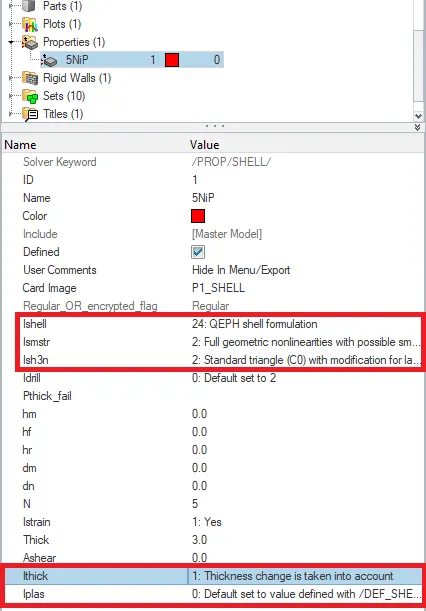
- The hourglass energy is constant through out the process. Because, the property card is assigned with the recommended values such as Ishell:24, Ismstr:2, Ish3n:2, Iplas:1, Ithick:1, N=5.
Case 2(Changing the values in failure card):-
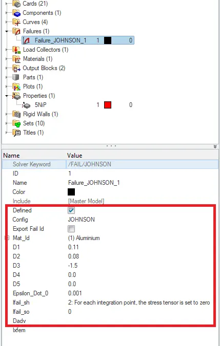
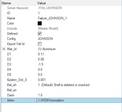
In this case, the failure card is edited with respect to the given values. But the material law is same(i.e., law 2). Before changing the values in the
failure card, it appears as shown in below fig. The values to be changed are Ifail_sh = 1, Dadv = 1, Ixfem = 1.
After changing the values in the failure card, it appears as shown in fig.
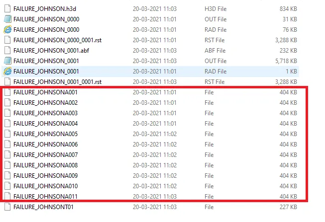
The next step is to run the simulation by using the radioss. After running the simulation, the obtained files(Animation files, time history files) in the
specified location appears as shown in fig.
The next step is to view the 0001.out file. Inorder to check for the energy errors, mass errors, etc. The 0001.out file with the maximum values are
shown in fig.
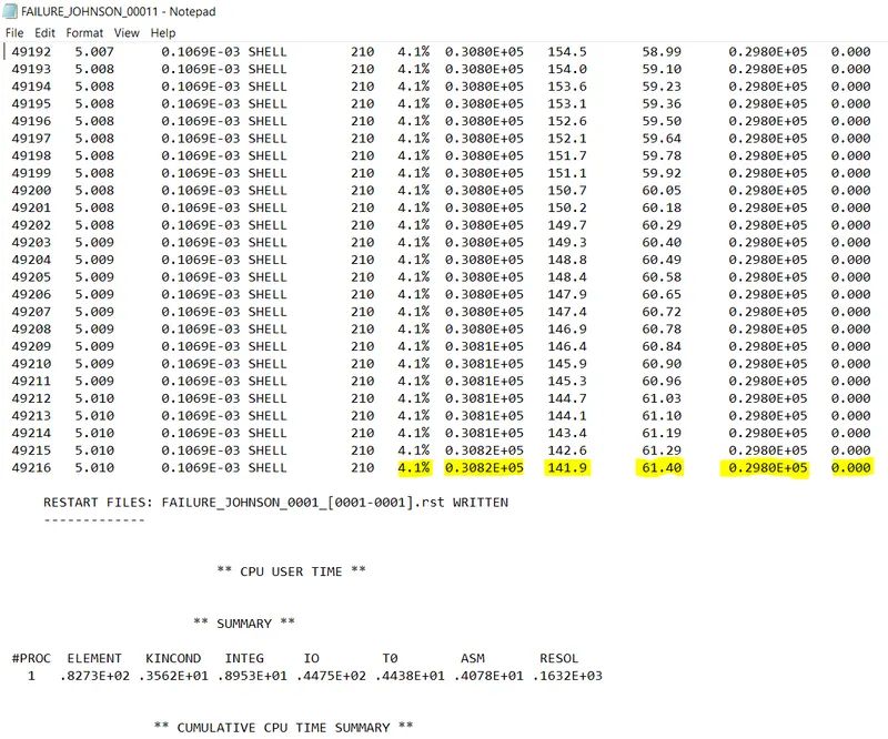
The obtained last cycle values are:
energy error = 4.1%
Internal energy = 0.3082E+05 KJ
Kinetic energy = 141.9 KJ
External work = 0.2980E+05 KJ
Mass error = 0
elapsed time = 49.60 s
Total number of cycles = 49217
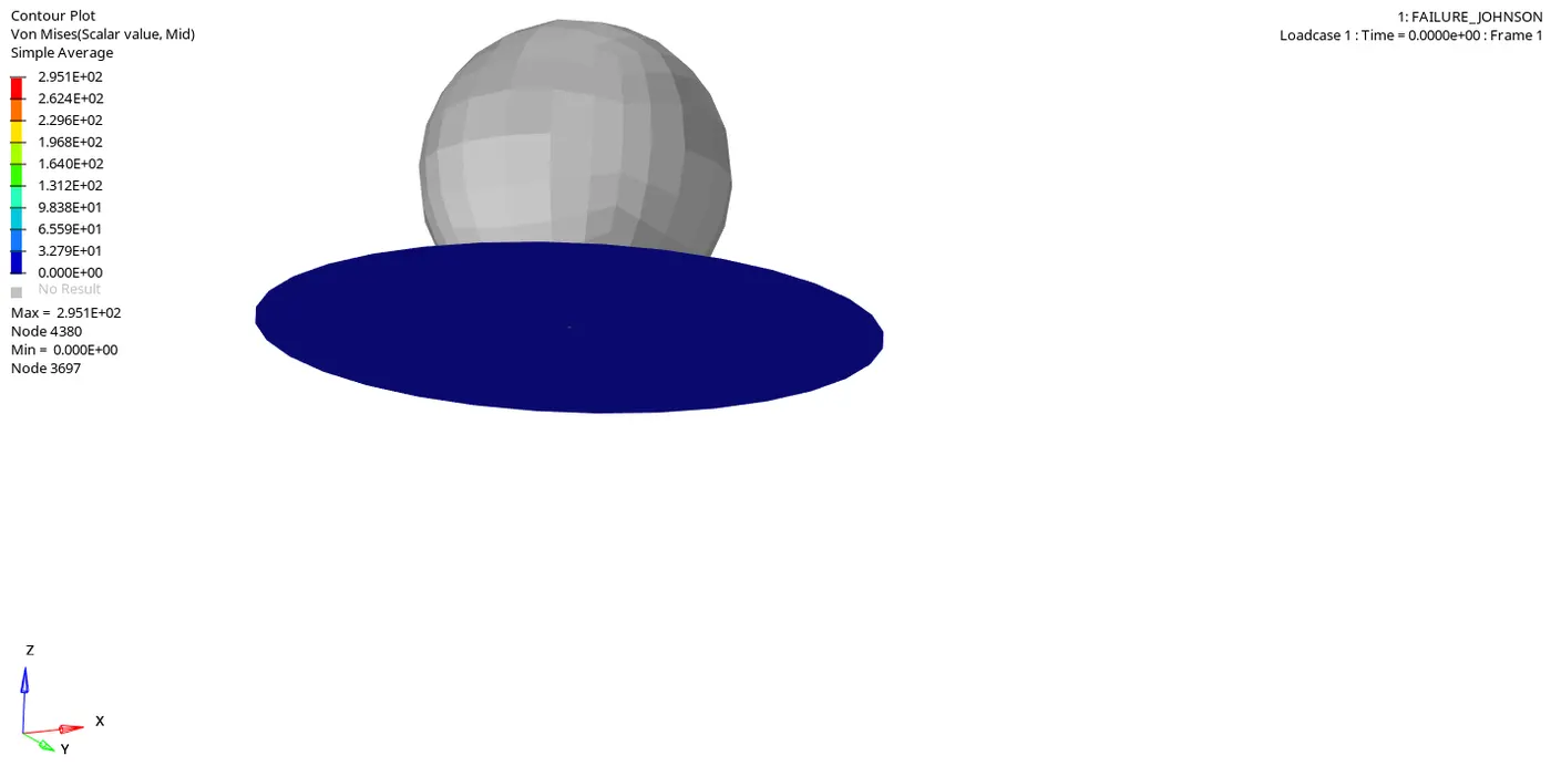
The obtained h3d file is imported in the hyperview, inorder to simulate. The obtained simulation appears as shown in the below animation.
Post-processing:
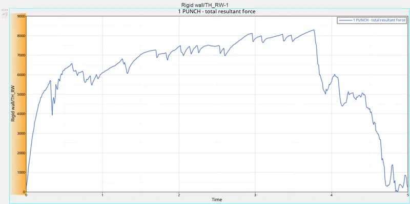
The obtained rigid wall foce is represented in the form of a graph as shown in fig. The total resultant force reches to a peak value due to the
impact of the rigid sphere towards the circular plate.
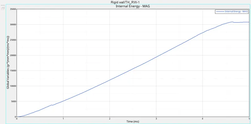
The obtained graph for internal energy appears as shown in fig. As usually, the internal energy starts from the origin & the reaches to the peak
value & after the breakage of elements, it reduces by a bit as shown in fig.
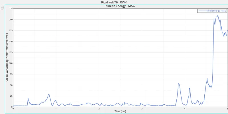
The obtained kinetic energy graph appears as shown in fig. Here the kinetic energy starts varying right from the beginning.
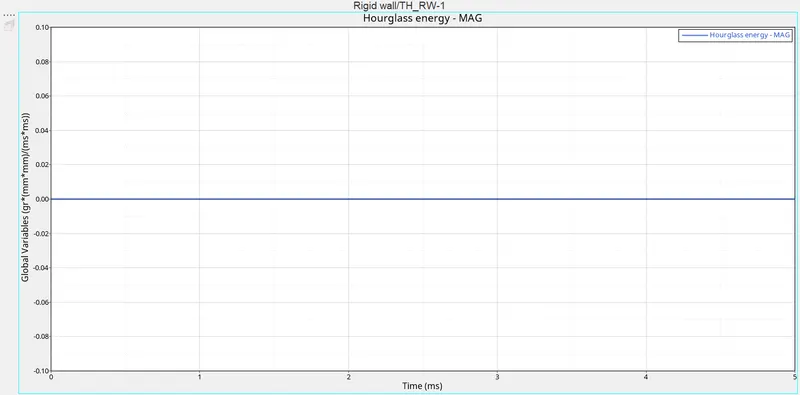
As the property assigned is with the recommended parameters such as the QEPH element with Ishell:24 is used, there will be no hourglass
energy(Because, it will have integrated hourglass enenrgy). So, the hourglass energy is constant as shown in fig.
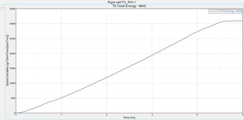
Total energy increases with the increase in internal energy & kinetic energy. The obtained total energy appears as shown in fig.
The contact energy also remains constant in all of the cases. Because the contacts are not specified.
Case 3(Deleting the failure johnson card):-
In this case, the failure card as shown in fig is deleted to see any changes in the result.
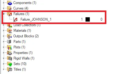
After deleting that card, the remaining cards appears as shown in fig.
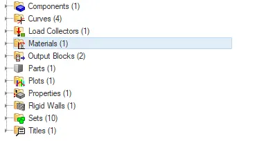
Now, the simulation is runned without changing any further parameters. After running it, the files obtained in the saved location.
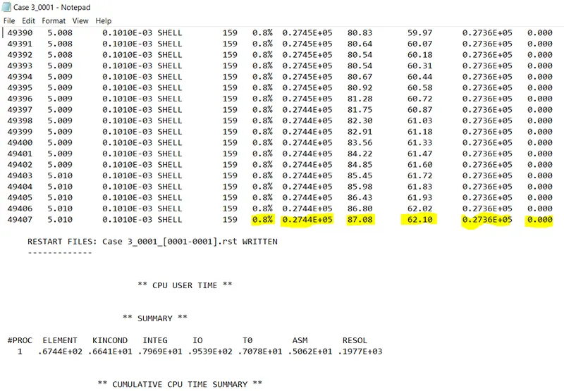
Then by opening the 0001.out file energy errors, mass errors, etc. The 0001.out file with the maximum values are shown in fig 5.32.
The obtained maximum values are:
energy error = 0.8%
Internal energy = 0.2744E+05 KJ
Kinetic energy = 87.08 KJ
External work = 0.2736E+05 KJ
Mass error = 0
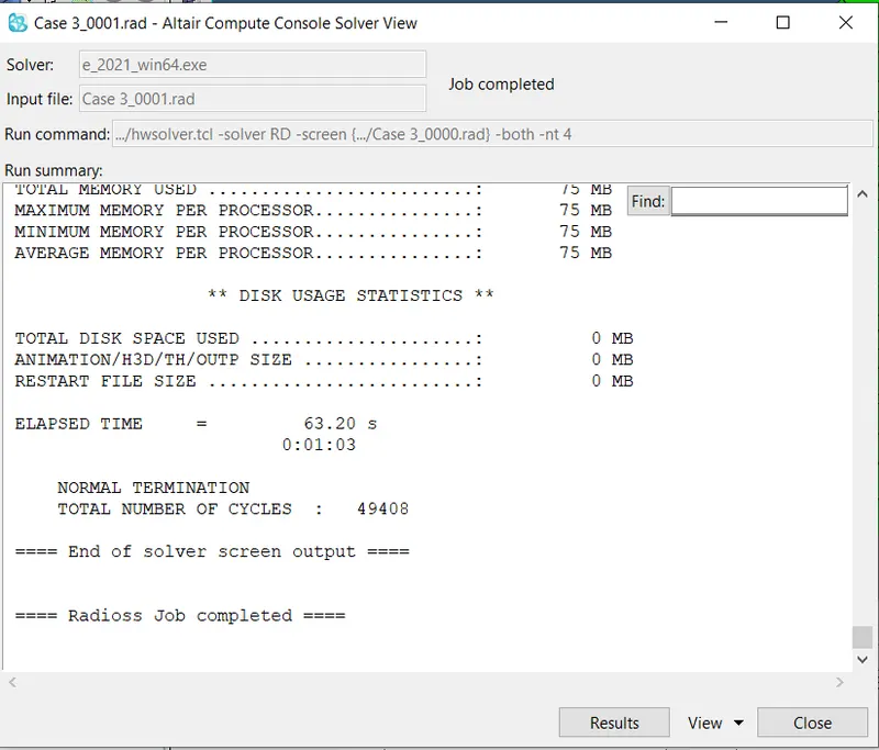
elapsed time = 63.20 s
Total number of cycles = 49408
Then the obtained h3d file is imported in the another window, In order to view the simulation. The obtained simulation in terms of von-mises is
shown in below animation.
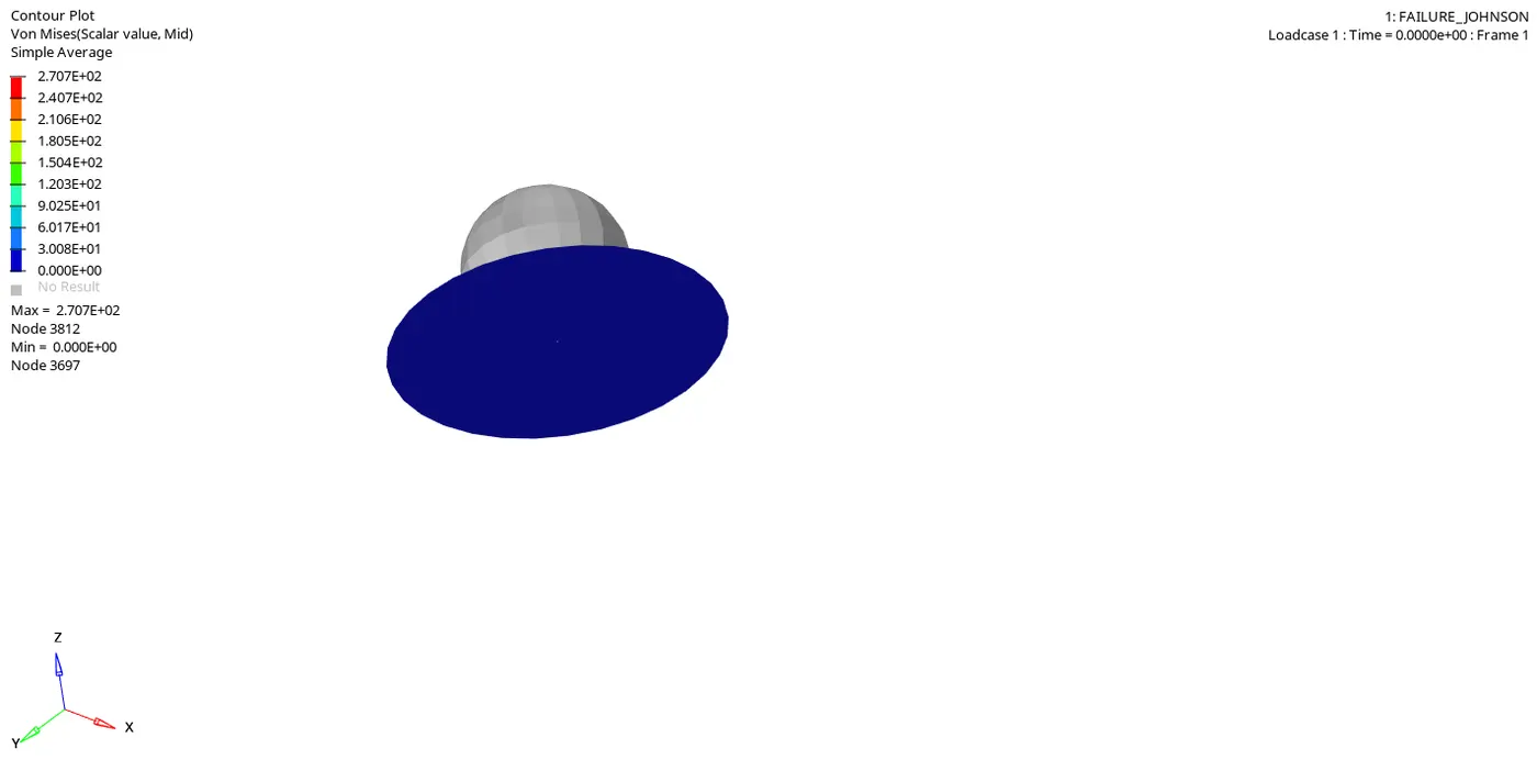
From the above animation, noticed thing is that, the elements break because, the circular plate is assigned with elasto-plastic material.
Post-processing:
The next step is to view the results, by the obtained graphs. These graphs are obtained by importing the obtained T01 file in the next window.
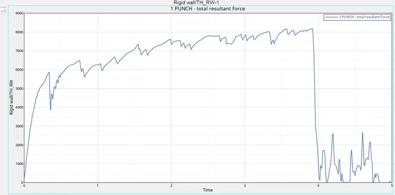
Initially, the rigid wall forces are obtained. The obtained graph is shown in fig.
Then the internal energy is plotted, it appears as shown in fig. This will be some what similar to the previous cases.
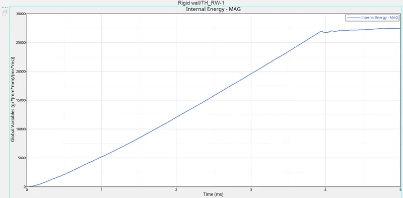
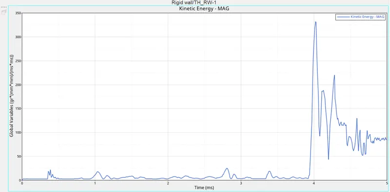
Then the kinetic energy graph is obtained, which appears as shown in fig. In this case the obtained kinetic energy will be some what less when
compared to the case 2.
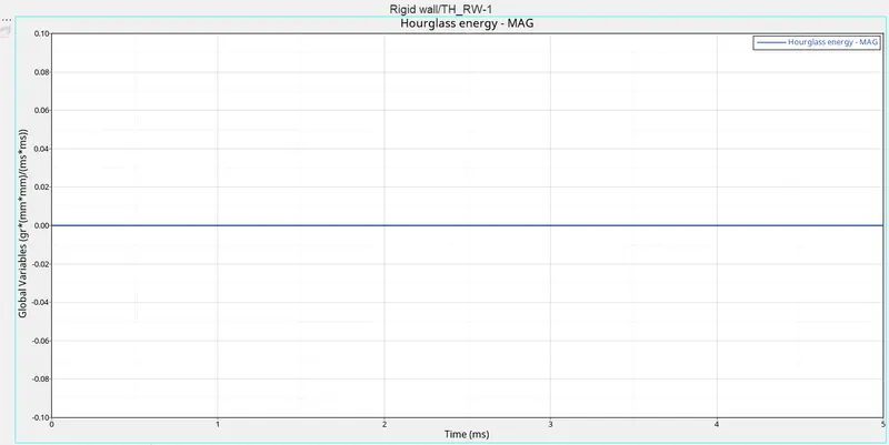
As the property assigned is with the recommended parameters such as the QEPH element with Ishell:24 is used, there will be no hourglass
energy(Because, it will have integrated hourglass enenrgy). So, the hourglass energy is constant as shown in fig.
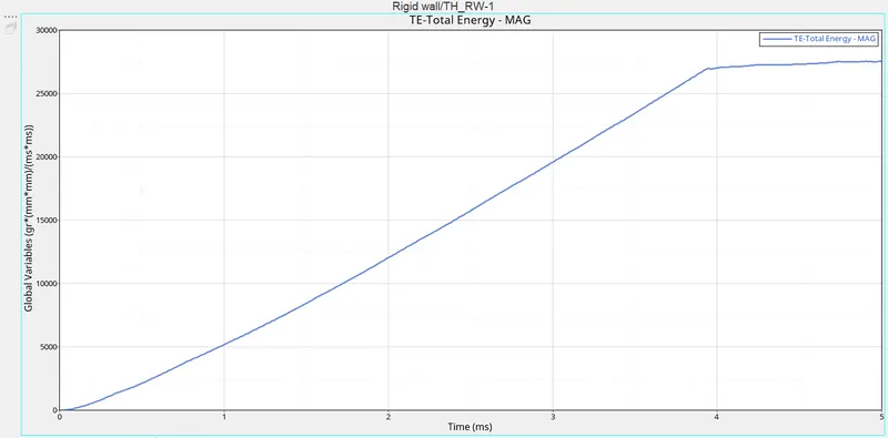
Total energy increases with the increase in internal energy & kinetic energy. The obtained total energy appears as shown in fig.
Case 4(Deleting the eps_max value from the material card):-
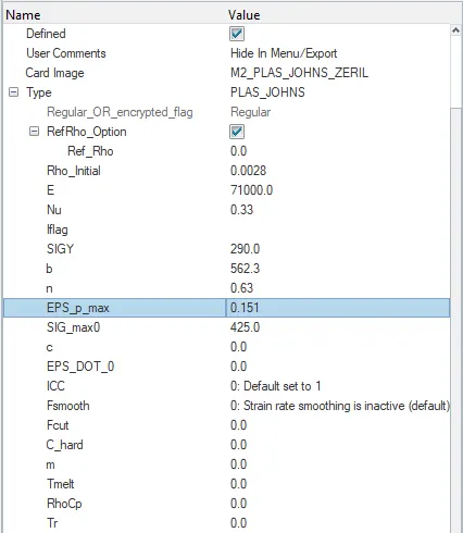
In this case for the same material card, the plastic strain(eps_max) value which is 0.151 as shown in fig, is removed(eps_max).
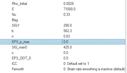
After removing the value for plasic strain, the material card appears as shown in fig.
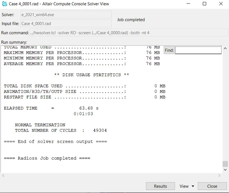
Then the simulation is runned using radioss. After running the obtained animation files stored in the specified location appears.
Then the obtained 0001.out file is opened. In order to view the obtained results in the form of values. The obtained values for last cycles are
shown in fig.
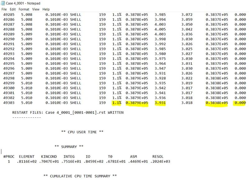
The obtained last cycle values are:
energy error = 1.1%
Internal energy = 0.3879E+05 KJ
Kinetic energy = 3.931 KJ
External work = 0.3838E+05 KJ
Mass error = 0
elapsed time = 63.68 s
Total number of cycles = 49304
Then the obtained h3d file is imported in the another window, In order to view the simulation. The obtained simulation in terms of von-mises is
shown in below animation. As the eps_max value (plastic strain) is zero, the elements will not break.
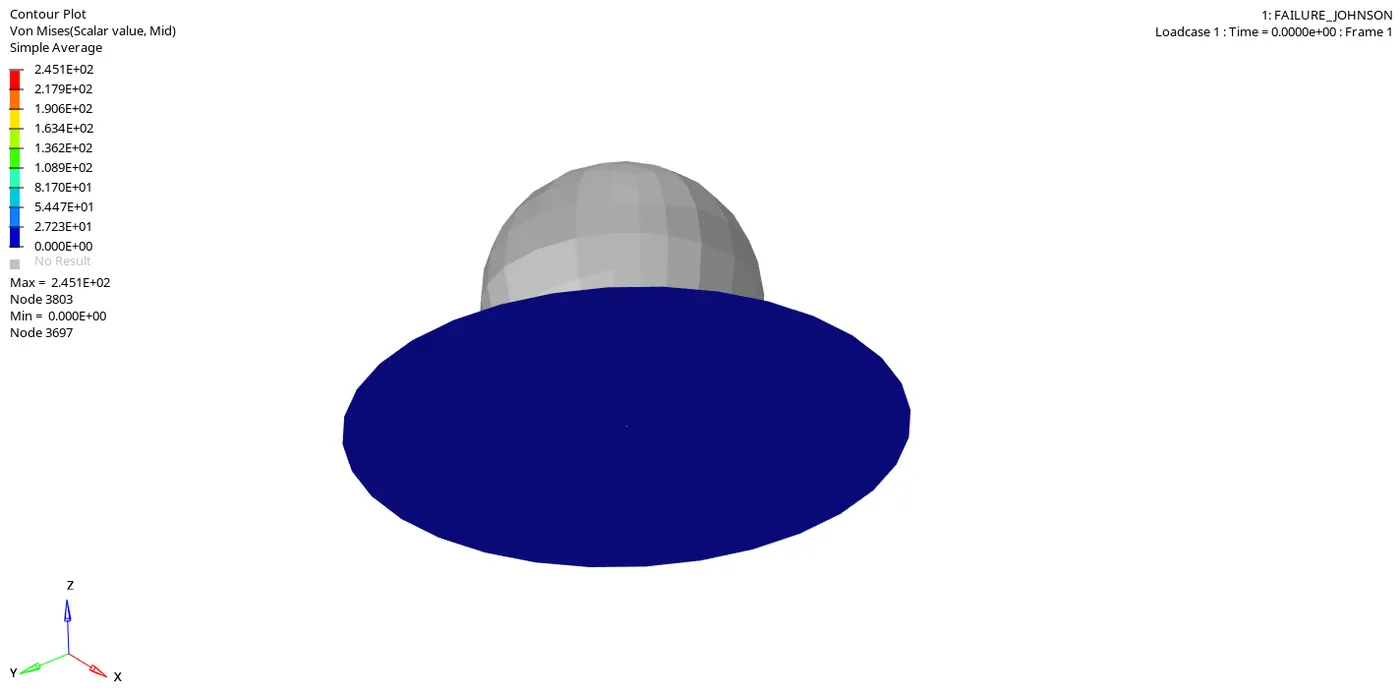
The elements are not getting deleted.
Post processing:
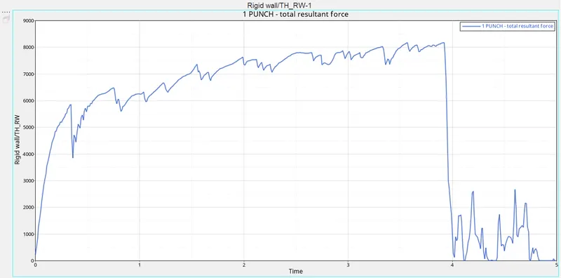
The obtained rigid wall force graph appears as shown in fig. The rigid wall force increases & decreases gradually. And reshes to the peak value at
the last moment of collision & decreases.
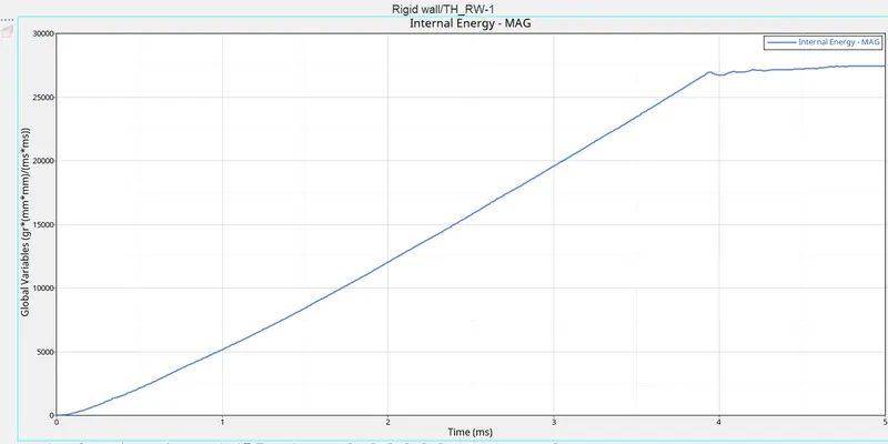
Then the internal energy is plotted, it appears as shown in fig. This will be some what similar to the previous cases.
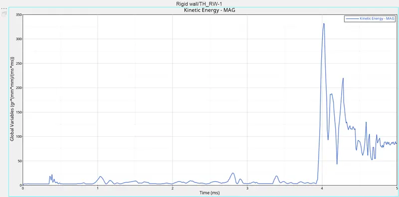
The obtained kinetic energy is plotted as shown in fig. And is similar to that of previus cases.
As the property assigned is with the recommended parameters such as the QEPH element with Ishell:24 is used, there will be no hourglass
energy(Because, it will have integrated hourglass enenrgy). So, the hourglass energy is constant as shown in fig.
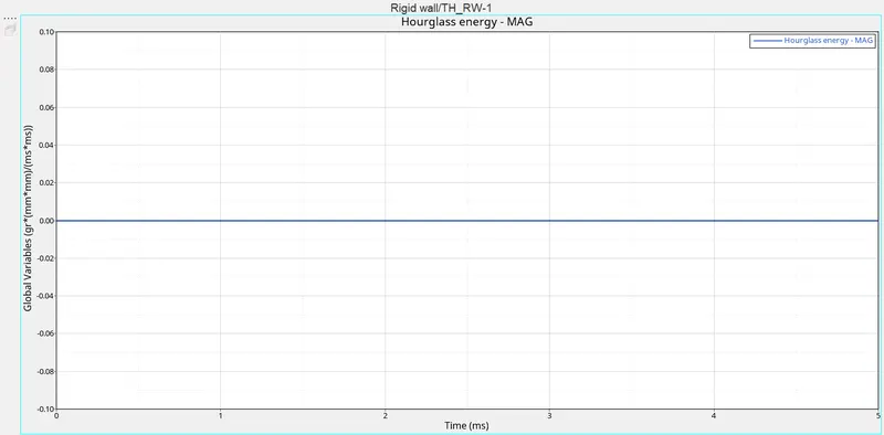
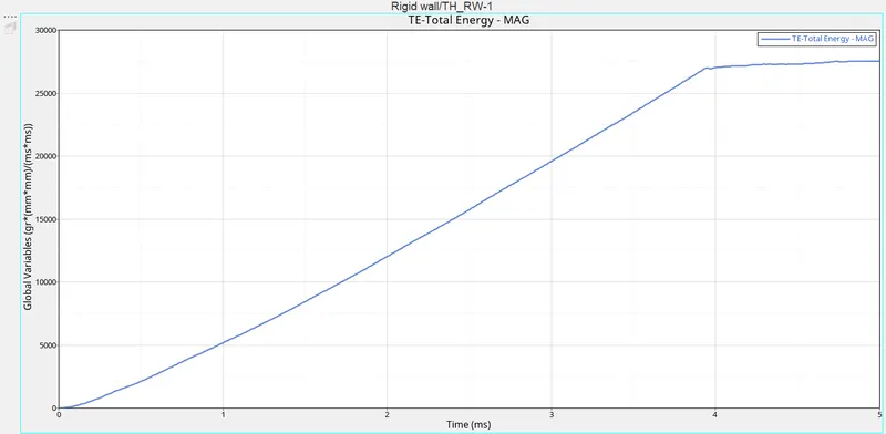
The obtained total energy graph appears as shown in fig. The total energy follows the internal energy & kinetic energy. So, there will be an
increase in total energy.
Case 5(Changing the material card to law 1):-
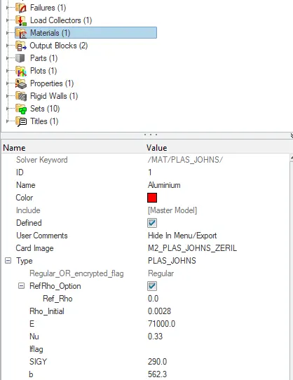
In this case, the material law is changed to law 1, which possess only the elastic behavior. Before changing the material law, it was in material law
2, as shown in fig.
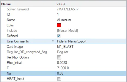
After changing the material card, it appears as shown in fig. And the values of E, ρ">ρρ, μ">μμ will remain the same.
Then the simulation is runned. After running the smulation, the obtained animation files appears in the same folder.
Then the obtained 0001.out file is opened, inorder to view the energy errors, mass errors. The obtained values are shown in fig.
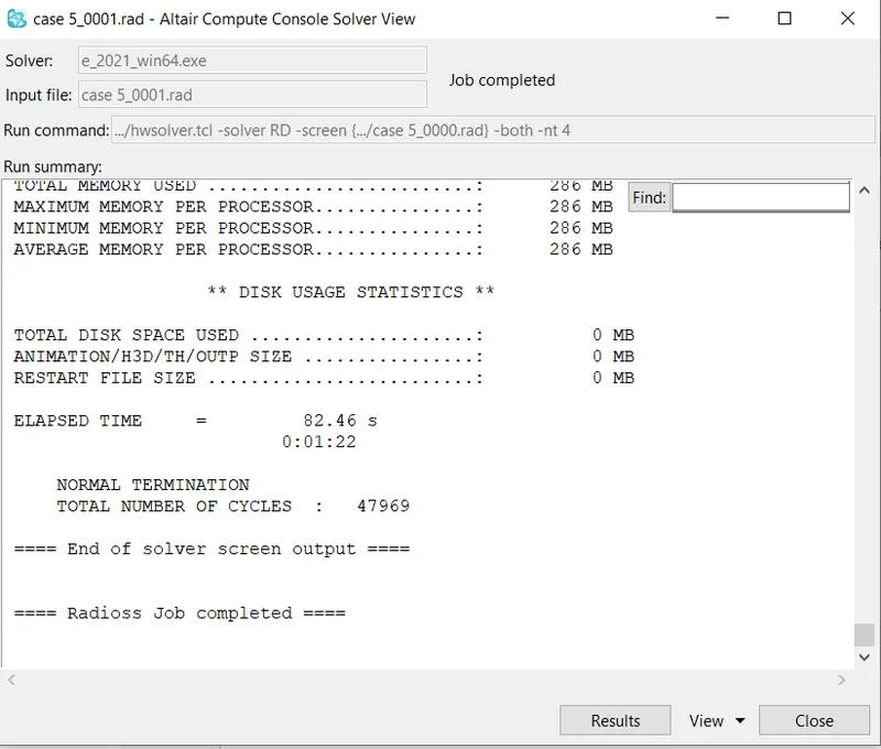
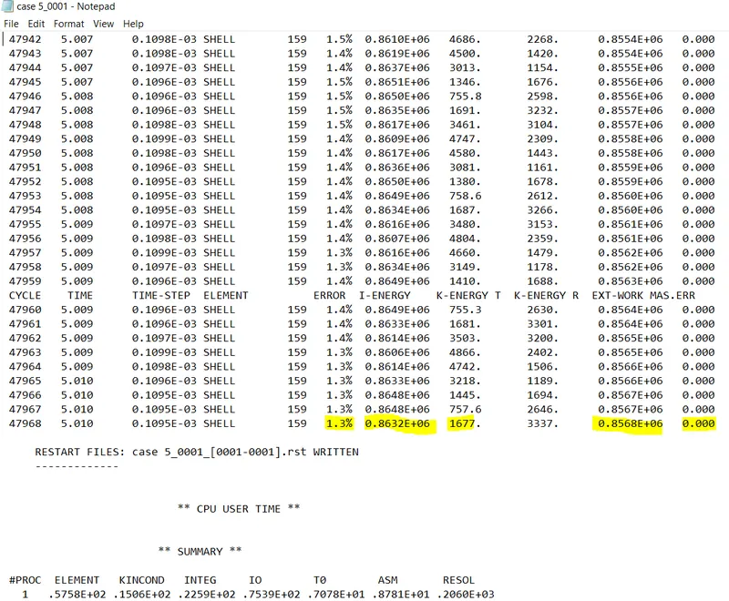
The obtained values for last cycle are:
energy error = 1.3%
Internal energy = 0.8632E+06 KJ
Kinetic energy = 1677 KJ
External work = 0.8568E+06 KJ
Mass error = 0
elapsed time = 82.46 s
Total number of cycles = 47969
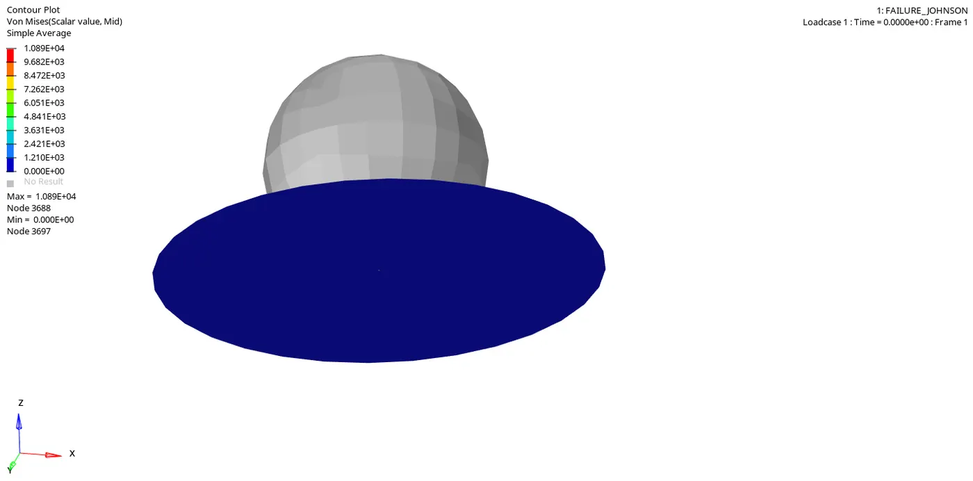
Then the obtained h3d file is imported in the another window, In order to view the simulation. The obtained simulation in terms of von-mises is
shown in below animation. The elements will not even split during the collision. Because, the law 1 is assigned to the circular plate. So, it possess
the elasticity (i.e., abitlity to regain its original size & shape).
Post-processing:
Then the graphs are plotted to view the results. The total resultant force of the rigid wall force increases gradually till the end. Because, there is no
plastic behavior seen in this case. The obtained rigid wall force graph appears as shown in fig.
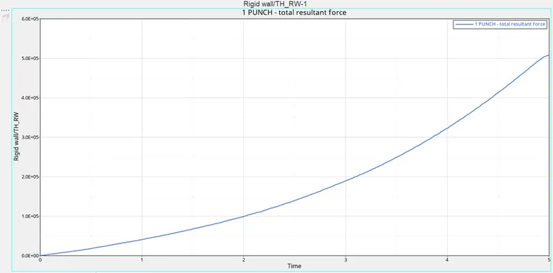
Then the internal energy graph is obtained, as shown in fig. Internal energy also increases gradually. But the graph will be some what
dissimilar to that of the previous cases.
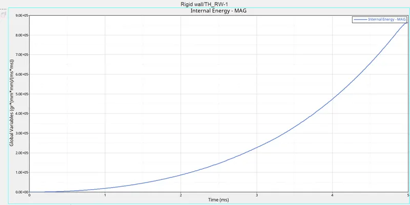
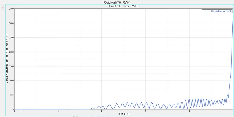
Then the kinetic energy is plotted, appears as shown in fig. Initially, the kinetic energy is constant. And it varies when the rigid sphere hits
the circular plate & it reaches to the peak value when the elements absorbs the more energy at the end of collision.
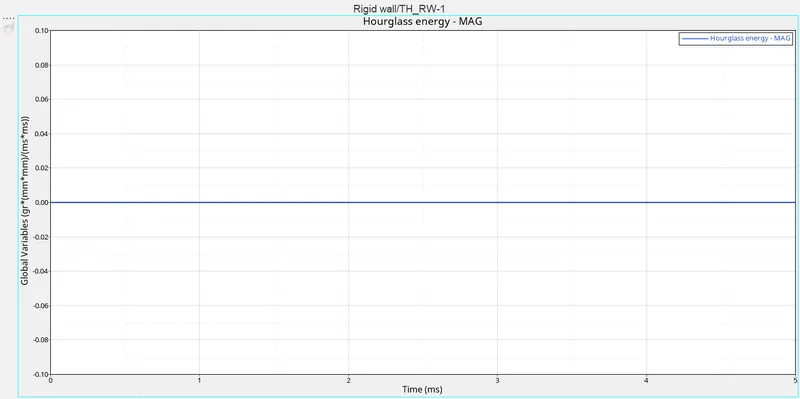
As the property assigned is with the recommended parameters such as the QEPH element with Ishell:24 is used, there will be no hourglass
energy(Because, it will have integrated hourglass enenrgy). So, the hourglass energy is constant as shown in fig.
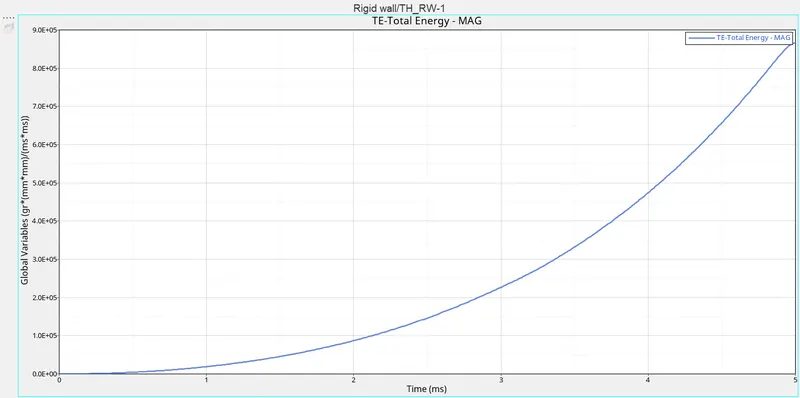
Total energy increases with the increase in internal energy & kinetic energy. The obtained total energy appears as shown in fig. And it keeps
on increasing just similar to the internal energy. And the graphvaries when compared to the other cases.
Case 6(Changing the material card to law 36 & parameters in the properrty card):-
In this case, the material card is changed to law 36(possess elasto-plastic piecewise linear material). And the shell parameters in the property card
are changed to the recommended properties. Before changing the parameters, the property card appears as shown in fig.
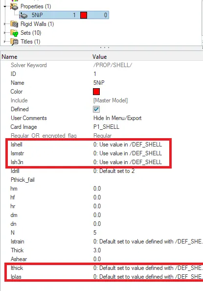
After changing the values, the material card appears as shown in fig.
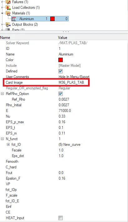
While defining the material card as law 36, a function should be represented to define the curves. Initially, there will be some curves are defined.
But a new curve is defined, the values are given by the user as shwon in fig. A curve will be generated based on the given values.
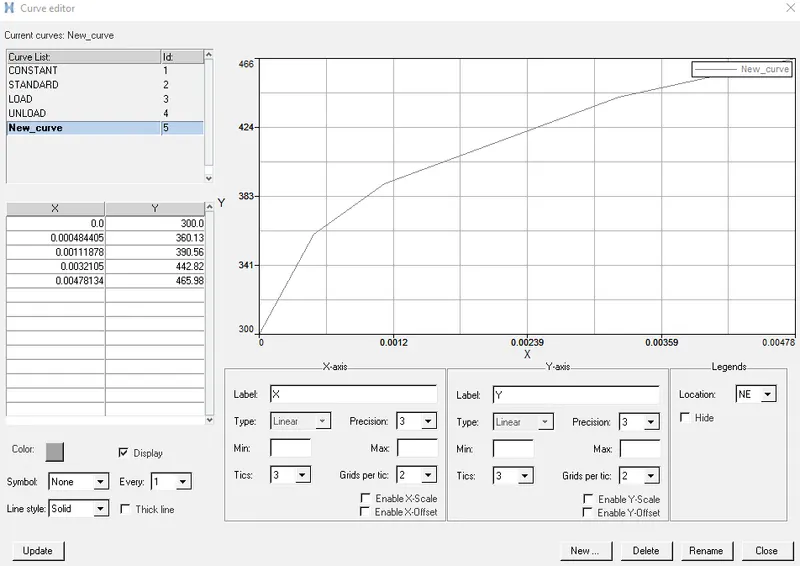
Higher the curve---> Higher the strain rate---> But earlier the failure takes place.
The process of creating the curve is: create---> curve---> New---> assign a name---> proceed---> shows the curve with values & graph.
Then the simulation is runned, by using radioss. After running the simulation, the 0001.out file is opened to view the obtained results in the form
of values, as shown in fig.
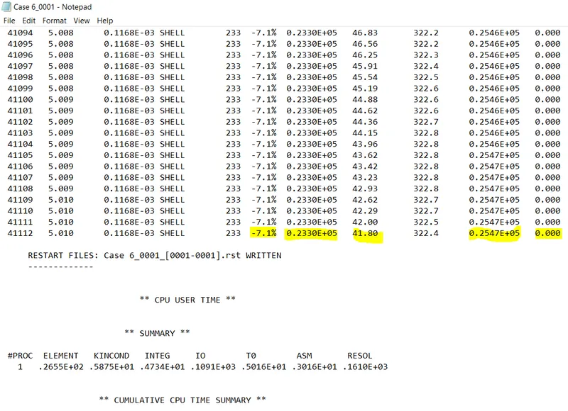
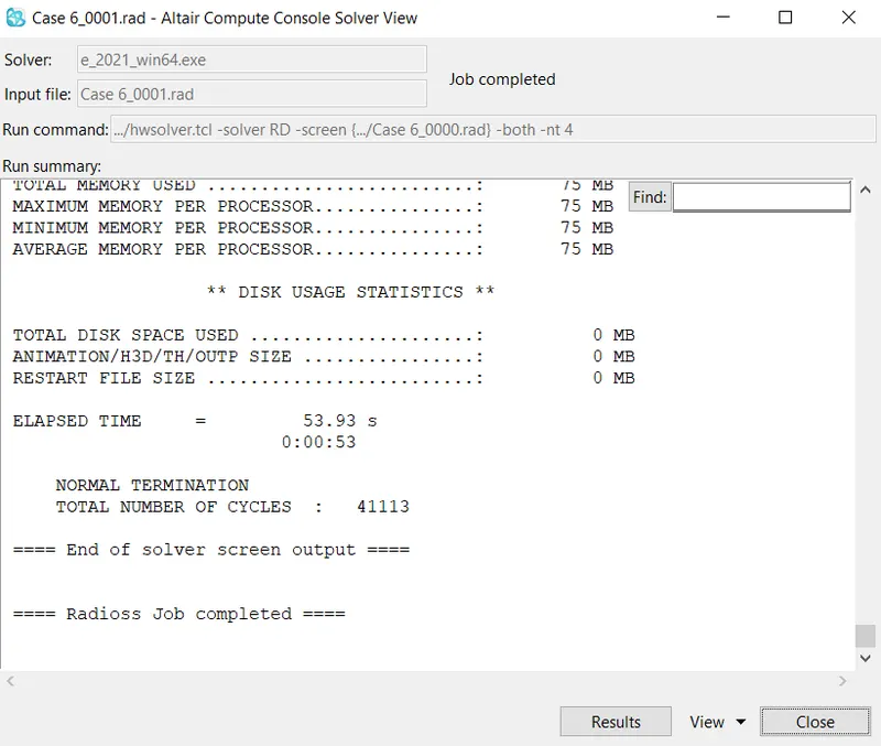
The obtained values for last cycle are:
energy error = -7.1%
Internal energy =0.2330E+05 KJ
Kinetic energy = 41.80 KJ
External work = 0.2547E+05 KJ
Mass error = 0
elapsed time = 53.93 s
Total number of cycles = 41113
Then the obtained h3d file is imported in the another window, In order to view the simulation. The obtained simulation in terms of von-mises
is shown in below animation.
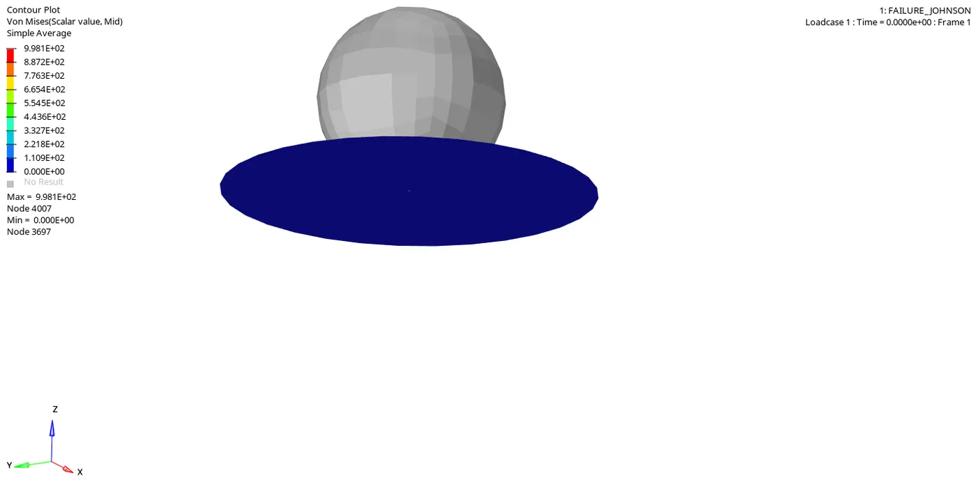
In this case also the elements will break. Beacuse, the material card assigned possess both elastic & plastic material.
Post-processing:
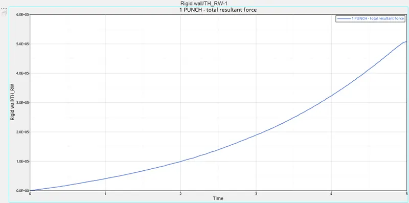
The rigid wall forces obtained are shown in the form of graph as shown in fig.
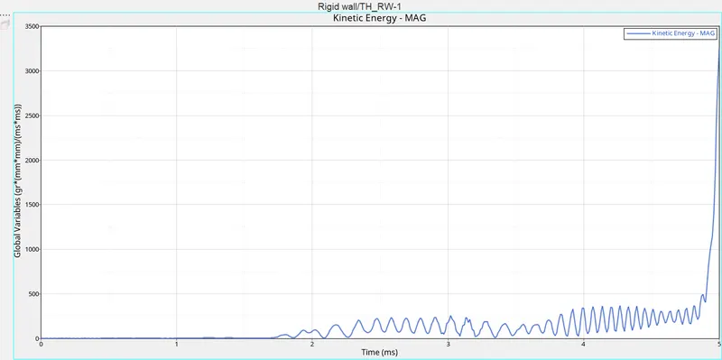
The obtained internal energy in the form of graph appears as shown in fig. The internal energy increases gradually same as in previous
case.
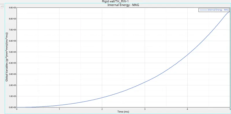
Then the obtained kinetic energy graph is plotted, shown in fig.
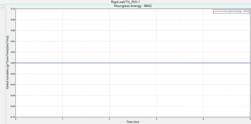
As the property assigned is with the recommended parameters such as the QEPH element with Ishell:24 is used, there will be no hourglass
energy(Because, it will have integrated hourglass enenrgy). So, the hourglass energy is constant as shown in fig.
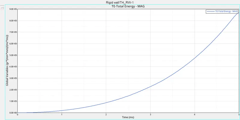
Total energy increases with the increase in internal energy & kinetic energy. The obtained total energy appears as shown in fig. And it keeps
on increasing just similar to the internal energy.
Case 7(Changing the material card to law 27):-
In this case, the material card is changed to law 27(Which possess brittleness) & to change the parameters in the property card with the
recommended values. For example: like aluminium & glass etc. This law combines the elasto-plastic johnson-cook material with an
orthographic brittle failure model. Before changing the parameters, the property card appears as shown in fig.
After changing the parameters in the property card, it appears as shown in fig.
Then the simulation is runned. After running the simulation, the obtained animation files in the specified location appears as shown in fig.
Then the 00001.out file is opened, inorder to view the energy errors, mass errors. The obtained values are shown in fig.
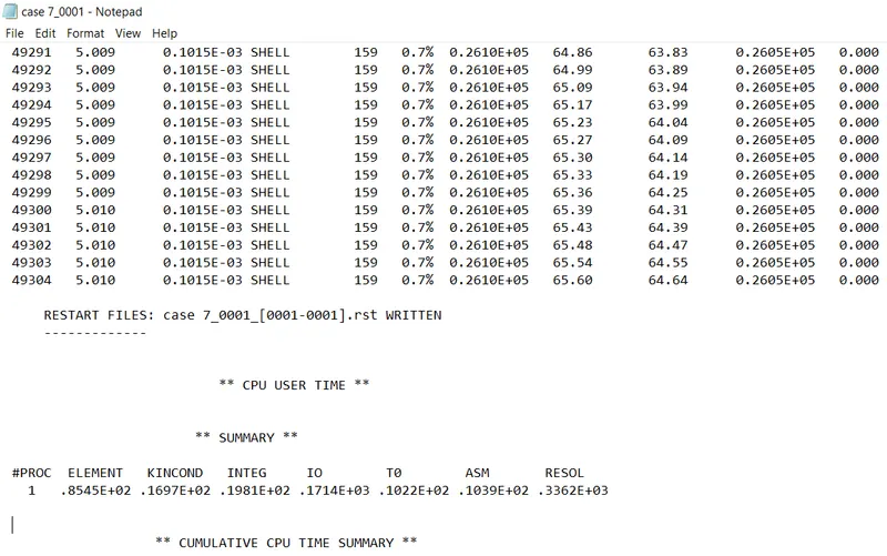
The obtained values for last cycle are:
energy error = 0.7%
Internal energy = 0.2610E+05 KJ
Kinetic energy = 65.60 KJ
External work = 0.2605E+05 KJ
Mass error = 0
elapsed time = 125.70 s
Total number of cycles = 49305
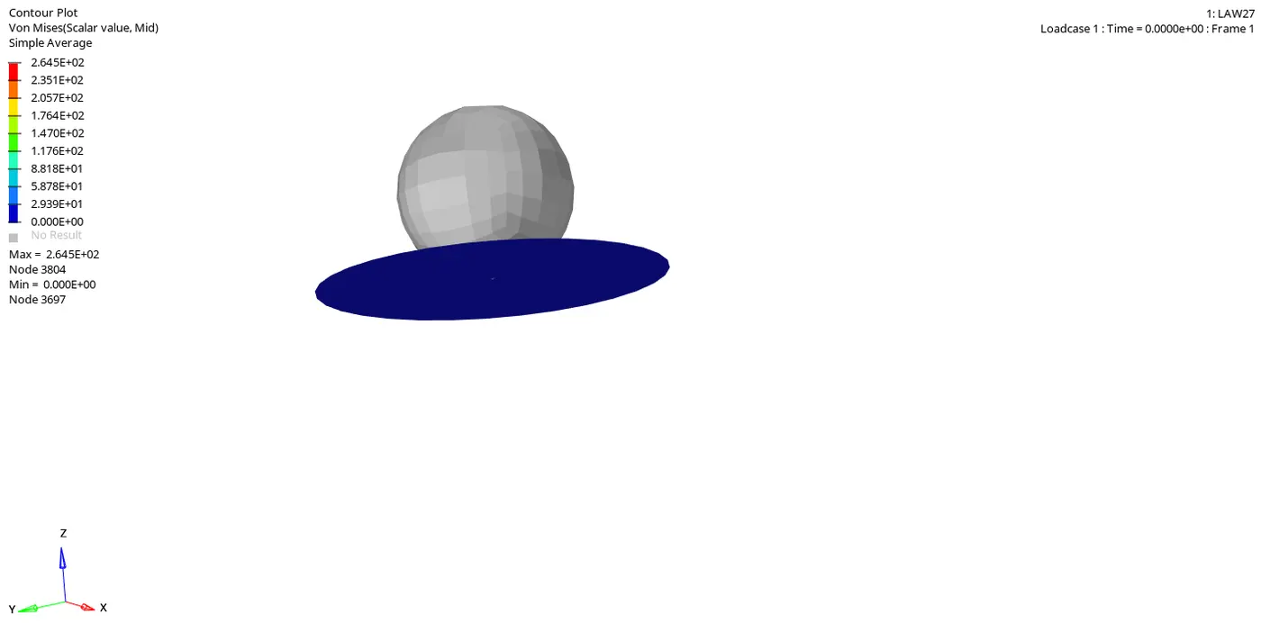
Then the obtained h3d file is imported in the another window, In order to view the simulation. The obtained simulation in terms of von-mises
is shown in below animation. Here the elements will break due to its brittle property.
Post-processing:
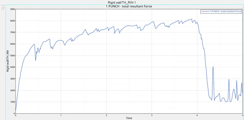
The obtained rigid wall forces graph appears as shown in fig. The rigid wall forces will reach a peak value at the time of impact and
decreases gradually.
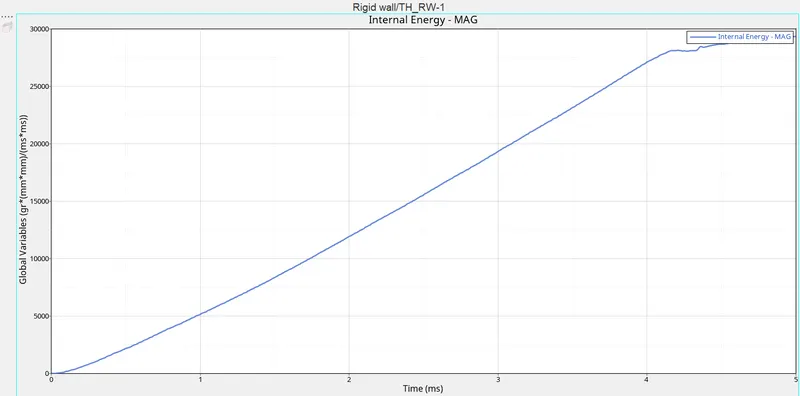
Then the obtained internal energy is plotted, as shown in fig.
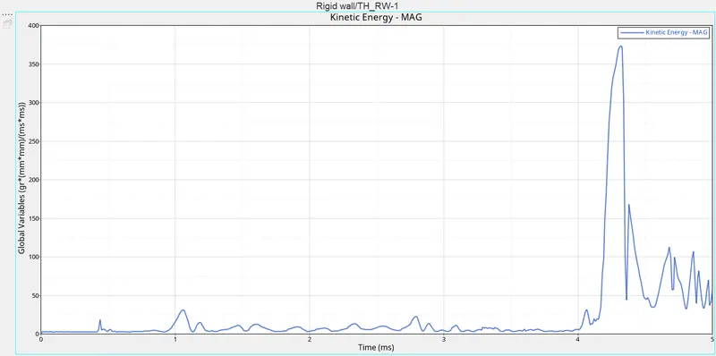
The obtained kinetic energy is plotted, shown in fig.
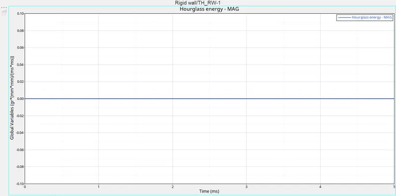
As the property assigned is with the recommended parameters such as the QEPH element with Ishell:24 is used, there will be no hourglass
energy(Because, it will have integrated hourglass enenrgy). So, the hourglass energy is constant as shown in fig.
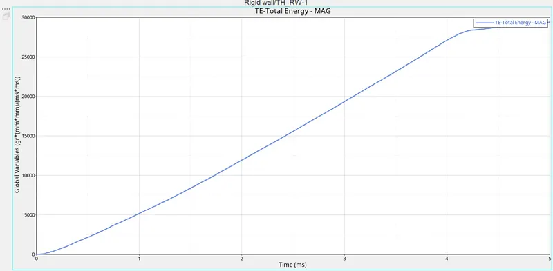
Total energy increases with the increase in internal energy & kinetic energy. The obtained total energy appears as shown in fig. And it
keeps on increasing just similar to the internal energy.
Comparsion of 7 cases:
| Basis of comparsion | case 1 | case 2 | case 3 | case 4 | case 5 | case 6 | case 7 |
| energy error(%) | 0.8% |
4.1% |
0.8% |
1.1% |
1.3% |
-7.1% |
0.7% |
| Internal energy(KJ) | 0.2730E+05 | 0.3082E+05 | 0.2744E+05 | 0.3879E+05 | 0.8632E+06 | 0.2330E+05 | 0.2610E+05 |
| Kinetic energy(KJ) | 67.81 | 141.9 | 87.08 | 3.931 | 1677 | 41.80 | 65.60 |
| External work(KJ) | 0.2721E+05 | 0.2980E+05 | 0.2736E+05 | 0.3838E+05 | 0.8568E+06 | 0.2547E+05 | 0.2605E+05 |
| Mass error | 0 | 0 | 0 | 0 | 0 | 0 | 0 |
| elapsed time(S) | 46.74 | 49.60 | 63.20 | 63.68 | 82.46 | 53.93 | 125.70 |
| Total number of cycles | 49380 | 49217 | 49408 | 49304 | 47969 | 41113 | 49305 |
| Elements deletion | will be deleted | will be deleted | will be deleted | will not be deleted | will not be deleted | will be deleted | will be deleted |
| Material law used |
Law 2 with a, b,n values |
Law 2 by changing the value in failure card |
Law 2 by deleting the failure johnson card |
Law 2 by removing plastic strain(eps_max) value | Law 1 | Law 36 | Law 27 |
6. Conclusion:
- Applied the various cases as mentioned in the above question on the given failure johnson cook material.
- Plotted the graphs(Post-processing) with respect to the obatined values from those cases.
- Finally, compared the obtained results from those cases.